Data analysis transforms raw data into meaningful insights. Graph Neural Networks take this a step further by handling complex relationships within data. In this comprehensive guide, I will explain how GNNs work and their applications in data analysis. You will learn the basics of GNNs, explore their benefits, and discover practical examples.
Understanding Graph Neural Networks
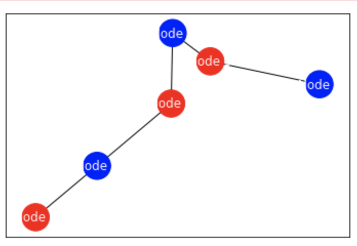
Fig.1 Schematic representation Graph Neural Networks which use nodes representing entities and edges representing relationships
Graph Neural Networks (GNNs) process data structured as graphs. Unlike traditional neural networks, which handle data in regular formats like arrays or matrices, GNNs excel with irregular data types. A graph consists of nodes (representing entities) and edges (representing relationships) as shown in fig.1.
The concept of GNNs emerged from the need to analyze graph-structured data efficiently. Researchers sought methods to capture dependencies among nodes in graphs, leading to the development of GNNs. This approach gained traction due to its ability to model complex relationships and interactions in data.
The significance of GNNs lies in their versatility. They can be applied to various domains such as social networks, biological networks, and recommendation systems. By leveraging the structure of graphs, GNNs can uncover patterns and insights that traditional methods might miss. Understanding GNNs opens new avenues for tackling complex data analysis challenges.
Key Concepts in GNNs
- Node Embeddings: GNNs create embeddings for nodes, representing them in a continuous vector space. These embeddings capture the node’s features and its neighborhood’s information.
- Message Passing: Nodes exchange information with their neighbors through message-passing mechanisms. Each node updates its state based on the messages received from adjacent nodes. This process iterates through multiple layers, allowing information to flow across the graph.
- Aggregation Functions: GNNs use aggregation functions to combine information from neighboring nodes. Common aggregation methods include mean, sum, and max pooling. These functions ensure that the model captures essential patterns from the graph structure.
Implementation of GNN
Let’s use the DGL (Deep Graph Library) to implement the same key parts of Graph Neural Networks (GNNs) such as node embedding, message passing, and aggregation functions.
Setting Up the Environment
Ensure you have the required libraries:
pip install torch dgl
Example Case: A Simple Graph
We’ll use a small graph with four nodes and five edges
import dgl
import torch
import torch.nn as nn
import torch.nn.functional as F

# Define node features (4 nodes, each with 3 features)
node_features = torch.tensor([
    [1, 2, 3],
    [4, 5, 6],
    [7, 8, 9],
    [10, 11, 12]
], dtype=torch.float)

# Define edges (source, target)
edge_list = [(0, 1), (1, 0), (2, 1), (3, 2), (0, 3)]

# Create the DGL graph
g = dgl.graph(edge_list)
g.ndata['feat'] = node_features
Node Embedding
We’ll use a simple linear layer to transform the node features into embeddings.
class NodeEmbedding(nn.Module):
    def __init__(self, in_dim, out_dim):
        super(NodeEmbedding, self).__init__()
        self.linear = nn.Linear(in_dim, out_dim)

    def forward(self, features):
        return self.linear(features)

# Initialize the embedding layer
embedding_layer = NodeEmbedding(in_dim=3, out_dim=2)
node_embeddings = embedding_layer(g.ndata['feat'])
print("Node Embeddings:\n", node_embeddings)
Message Passing and Aggregation Function
DGL simplifies message passing and aggregation. We’ll use DGL’s built-in functions to implement these steps.
import dgl.function as fn
class MessagePassingLayer(nn.Module):
def __init__(self):
super(MessagePassingLayer, self).__init__()
def forward(self, g, node_embeddings):
# Use DGL's message passing API
g.ndata['h'] = node_embeddings
g.update_all(fn.copy_u('h', 'm'), fn.mean('m', 'h'))
return g.ndata.pop('h')
# Initialize the message passing layer
message_passing_layer = MessagePassingLayer()
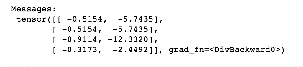
messages = message_passing_layer(g, node_embeddings)
print("Messages:\n", messages)
The output is as follow,
Combining Embeddings and Messages
After message passing, we will update the node embeddings by combining their original embeddings with the aggregated messages.
class GNNLayer(nn.Module):
def __init__(self, in_dim, out_dim):
super(GNNLayer, self).__init__()
self.embedding = NodeEmbedding(in_dim, out_dim)
self.message_passing = MessagePassingLayer()
def forward(self, g, features):
node_embeddings = self.embedding(features)
messages = self.message_passing(g, node_embeddings)
return node_embeddings + messages # Update node embeddings with aggregated messages
# Initialize the GNN layer
gnn_layer = GNNLayer(in_dim=3, out_dim=2)
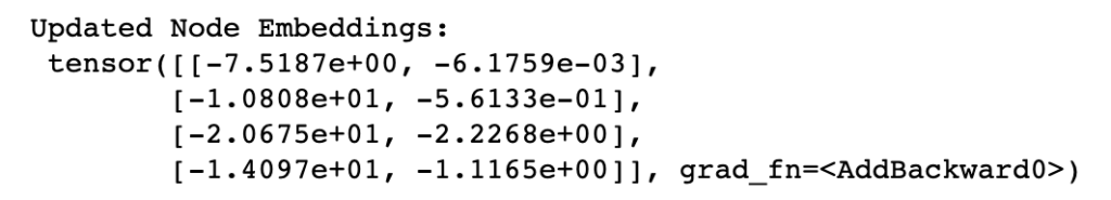
updated_embeddings = gnn_layer(g, g.ndata['feat'])
print("Updated Node Embeddings:\n", updated_embeddings)
The output is given below,
Stacking GNN Layers
We will stack multiple GNN layers to build a simple GNN model.
class SimpleGNN(nn.Module):
    def __init__(self, in_dim, hidden_dim, out_dim):
        super(SimpleGNN, self).__init__()
        self.layer1 = GNNLayer(in_dim, hidden_dim)
        self.layer2 = GNNLayer(hidden_dim, out_dim)

    def forward(self, g, features):
        x = self.layer1(g, features)
        x = F.relu(x)
        x = self.layer2(g, x)
        return x

# Initialize the GNN model
model = SimpleGNN(in_dim=3, hidden_dim=4, out_dim=2)
output = model(g, g.ndata['feat'])
print("Final Node Embeddings:\n", output)
The final output is;
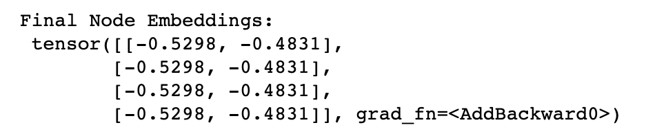
Explanation
- Node Embedding: The
NodeEmbeddingclass transforms initial node features into a lower-dimensional space, creating node embeddings. - Message Passing and Aggregation: The
MessagePassingLayerclass uses DGL’s built-in functions to aggregate information from neighboring nodes using mean pooling. - GNN Layer: The
GNNLayerclass combines the node’s own embedding with the aggregated messages to update its state. - SimpleGNN Model: The
SimpleGNNclass stacks two GNN layers, allowing for deeper feature extraction and transformation.
This implementation with DGL demonstrates the core components of GNNs: node embedding, message passing, and aggregation functions. You can extend this framework to more complex graphs and applications, leveraging the power of GNNs for various tasks.
Visualizing Node Embeddings in a Graph Using DGL and Matplotlib
To visualize the graph along with the node embeddings, we’ll use the networkx and matplotlib libraries. We’ll plot the graph with the node embeddings as node labels.
First, make sure you have the necessary libraries:
pip install networkx matplotlib
Define the GNN Components and Example Graph
import dgl
import torch
import torch.nn as nn
import torch.nn.functional as F
import networkx as nx
import matplotlib.pyplot as plt
import dgl.function as fn
# Define node features (4 nodes, each with 3 features)
node_features = torch.tensor([
[1, 2, 3],
[4, 5, 6],
[7, 8, 9],
[10, 11, 12]
], dtype=torch.float)
# Define edges (source, target)
edge_list = [(0, 1), (1, 0), (2, 1), (3, 2), (0, 3)]
# Create the DGL graph
g = dgl.graph(edge_list)
g.ndata['feat'] = node_features
class NodeEmbedding(nn.Module):
def __init__(self, in_dim, out_dim):
super(NodeEmbedding, self).__init__()
self.linear = nn.Linear(in_dim, out_dim)
def forward(self, features):
return self.linear(features)
class MessagePassingLayer(nn.Module):
def __init__(self):
super(MessagePassingLayer, self).__init__()
def forward(self, g, node_embeddings):
# Use DGL's message passing API
g.ndata['h'] = node_embeddings
g.update_all(fn.copy_u('h', 'm'), fn.mean('m', 'h'))
return g.ndata.pop('h')
class GNNLayer(nn.Module):
def __init__(self, in_dim, out_dim):
super(GNNLayer, self).__init__()
self.embedding = NodeEmbedding(in_dim, out_dim)
self.message_passing = MessagePassingLayer()
def forward(self, g, features):
node_embeddings = self.embedding(features)
messages = self.message_passing(g, node_embeddings)
return node_embeddings + messages # Update node embeddings with aggregated messages
class SimpleGNN(nn.Module):
def __init__(self, in_dim, hidden_dim, out_dim):
super(SimpleGNN, self).__init__()
self.layer1 = GNNLayer(in_dim, hidden_dim)
self.layer2 = GNNLayer(hidden_dim, out_dim)
def forward(self, g, features):
x = self.layer1(g, features)
x = F.relu(x)
x = self.layer2(g, x)
return x
# Initialize the GNN model
model = SimpleGNN(in_dim=3, hidden_dim=4, out_dim=2)
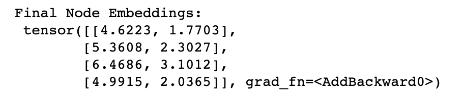
output = model(g, g.ndata['feat'])
print("Final Node Embeddings:\n", output)
The output is given below,
Visualize the Graph with Updated Node Embeddings
# Convert the DGL graph to a NetworkX graph
nx_graph = g.to_networkx().to_undirected()
# Extract the final node embeddings as labels
labels = {i: f"{output[i].detach().numpy()}" for i in range(output.shape[0])}
# Plot the graph
plt.figure(figsize=(8, 6))
pos = nx.spring_layout(nx_graph) # Position nodes using Fruchterman-Reingold force-directed algorithm
nx.draw(nx_graph, pos, with_labels=True, node_color='skyblue', node_size=700, font_size=10, font_color='black', edge_color='gray')
nx.draw_networkx_labels(nx_graph, pos, labels, font_size=10, font_color='red')
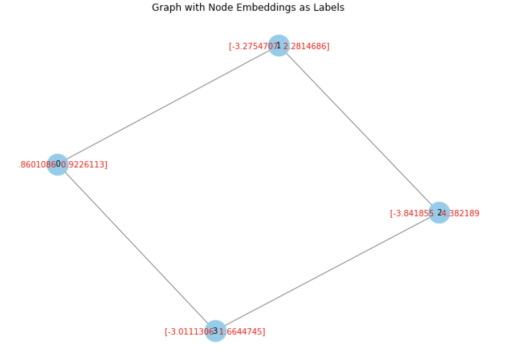
plt.title("Graph with Node Embeddings as Labels")
plt.show()
The final output is shown below,
Explanation
- Define the GNN Components and Example Graph: We define our graph, node features, and the GNN layers (NodeEmbedding, MessagePassingLayer, GNNLayer, and SimpleGNN).
- Initialize the GNN Model: We create an instance of
SimpleGNNand compute the final node embeddings. - Visualize the Graph with Updated Node Embeddings: We convert the DGL graph to a NetworkX graph for visualization. We extract the node embeddings and use them as labels on the nodes. We then plot the graph using Matplotlib, with the node embeddings displayed in red.
This code will output the graph with nodes labeled by their final embeddings, providing a clear visual representation of the embeddings learned by the GNN.
Challenges in Using GNNs for Data Analysis
While GNNs offer powerful tools for data analysis, they come with challenges:
Scalability
Graphs can grow large and complex. Handling massive graphs efficiently remains a challenge. Computational resources and memory limitations can constrain scalability.
Interpretability
GNNs often act as black-box models. Understanding how they make decisions can be difficult. Enhancing interpretability is crucial for trust and validation, especially in sensitive applications.
Data Quality
Graphs rely on accurate data. Noisy, incomplete, or incorrect data can degrade GNN performance. Ensuring high-quality graph data is essential for reliable analysis.
Model Complexity
Designing and tuning GNNs involves choosing appropriate architectures and hyperparameters. This complexity can make model development and optimization time-consuming and requires expertise.
Training Time
Training GNNs on large graphs can be slow. Efficient training algorithms and hardware accelerations, like GPUs, are necessary to speed up the process.
Despite these challenges, GNNs offer unique capabilities for analyzing structured data. Their ability to model relationships and dependencies makes them invaluable for various applications. As the field progresses, solutions to these challenges will enhance their applicability and performance.
Feel free to share your thoughts and comments on this blog topic.Subscribe to our website to stay connected!