Every model eventually faces the same trap. It fits the training data almost perfectly, yet it stumbles the moment you show it something new. This trap has a name: overfitting. And today, we meet the first real tool that fixes it: ridge regression.
This article walks through the companion video for Episode 36 of the Intelevo machine learning series. By the end, you will understand exactly what ridge regression does, why it works, and how to use it in just three lines of Python.
A Quick Recap: Why Curves Get Carried Away
In our last episode, we gave our regression model the power to bend. Polynomial regression added x², x³, and beyond, so a straight line could twist into a curve. That flexibility solved a real problem. However, it also introduced a new one.
A curve that bends too eagerly starts chasing everything in the training data, including the noise. It memorizes instead of learning. And once that happens, its predictions on fresh data become unreliable.
Here’s the surprising part. This overfitting rarely announces itself as a wiggly curve alone. Instead, it hides inside the numbers. Specifically, it shows up as coefficients that grow huge and extreme. Each one strains harder and harder to explain one tiny quirk in the data.
Consider a simple housing model. A well-behaved model might assign a coefficient of 42 to house size. An overfit version of that same model might assign it 1,847. Neither number is “wrong” in a mathematical sense. But the second one signals a model that has lost its grip on reality.
The Anchor Analogy: A Simple Way to Picture Ridge Regression
Let’s build a picture you can carry through this entire topic.
Imagine a small boat floating in choppy water. Waves represent the noise inside your data, and they push the boat in every direction. Without anything holding it back, the boat drifts wherever the last wave shoved it.
Now, drop an anchor. The boat can still move with real currents. Yet it resists those wild, noisy swings, and it settles closer to the center.
That anchor is exactly what ridge regression gives to your coefficients. Every coefficient gets its own gentle pull back toward zero. As a result, none of them can swing to an extreme value just because of one noisy data point.
What Ridge Regression Actually Does
In plain words, ridge regression starts as ordinary linear regression. Then, it adds one extra request: “please, keep your coefficients modest.”
The model still tries to fit the data as closely as it can. However, it now pays a penalty whenever a coefficient grows too large. So the goal quietly shifts. Instead of fitting the data as closely as possible, ridge regression fits the data well and stays modest at the same time.
This single shift changes everything about how the model behaves on new, unseen data.
The Only Formula You Need
Ridge regression introduces exactly one new idea into the math, and it’s simpler than it looks:
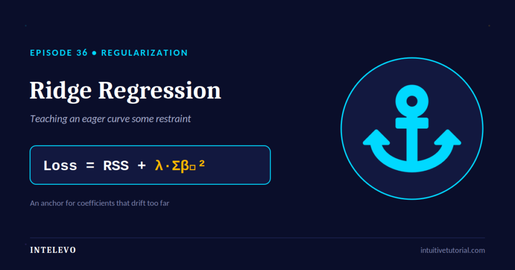
Loss = RSS + λ · Σβᵢ²
Let’s break this into three pieces.
RSS stands for the residual sum of squares. It measures the usual “how wrong were we” error, just like ordinary linear regression.
λ (lambda) is the new strictness knob. It decides how hard the model pulls on the anchor line. A small lambda means a gentle pull. A large lambda means a strong one.
Σβᵢ² adds up the square of every coefficient in the model. In other words, it measures the total “extremeness” of the entire coefficient set.
Put together, bigger coefficients now cost more. Therefore, the model only lets a coefficient grow large when the data truly earns it.
Choosing Lambda: The Strictness Knob
Lambda controls everything, so let’s look at what happens at each extreme.
When lambda equals zero, there’s no pull at all. The model behaves exactly like plain linear regression, and coefficients can still run wild.
When lambda sits at a moderate, well-chosen value, the model tames those extreme coefficients without losing the real pattern underneath the data.
When lambda grows too large, it pulls so hard that every coefficient flattens toward zero. At that point, the model underfits, and it misses the pattern entirely.
Consequently, the sweet spot never sits at either extreme. Instead, it sits wherever the anchor stays useful, without dragging the boat to a complete stop.
The Secret That Makes It Click
Here’s the detail that turns confusion into clarity.
Ridge regression shrinks every coefficient toward zero. It does this evenly, in proportion to each coefficient’s size. However, it never lets any coefficient hit exactly zero. The anchor line never goes fully slack.
Consequently, every feature stays inside the model. Each one simply becomes a quieter, more modest version of itself.
Keep this detail in mind. Our next episode explores what happens when we let that anchor line snap completely for some features.
Watching the Coefficients Shrink
Numbers make this idea concrete, so let’s compare two versions of the same housing model.
| Feature | Without Ridge | With Ridge (λ = 10) |
|---|---|---|
| Size (sq. ft.) | 1,847.30 | 38.40 |
| Bedrooms | −19,402.60 | −410.20 |
| Age of house | 6,733.90 | −95.60 |
| Distance to city | −58,910.10 | −1,220.80 |
Notice the pattern immediately. Every coefficient on the right sits dramatically closer to zero than its counterpart on the left. Yet none of them actually reach zero. That’s ridge regression working exactly as designed.
A Trade We’re Happy to Make
This shrinkage comes at a cost, and understanding that cost matters.
On one side, the model accepts a little more bias. Since the anchor prevents a perfect fit on training data, predictions shift slightly off center, on average.
On the other side, the model gains much less variance. Predictions stop swinging wildly whenever new data arrives. Instead, the model stays steady and reliable across many different samples.
In practice, this trade almost always pays off. A small, predictable dose of bias buys a much bigger drop in variance. And a model with low variance generalizes far better to the real world.
Python in Action: Three Lines to a Calmer Model
Let’s move from theory into code. Scikit-learn makes ridge regression remarkably simple to apply.
from sklearn.linear_model import Ridge

model = Ridge(alpha=10)
model.fit(X_train, y_train)

print(model.coef_)
# smaller, steadier numbers
Notice how little actually changes here. The model name switches from LinearRegression to Ridge. The parameter alpha plays the role of lambda from our formula; it controls the anchor’s pulling strength. Everything else, including .fit() and .predict(), works exactly like before.
Bonus: Letting Cross-Validation Pick Alpha for You
Manually guessing the right alpha wastes time. Instead, try a handful of values and check which one predicts new, unseen data best.
from sklearn.linear_model import RidgeCV
import numpy as np

alphas = np.array([0.01, 0.1, 1, 10, 50, 100, 500])
model = RidgeCV(alphas=alphas, store_cv_values=True)
model.fit(X_train, y_train)

print(model.alpha_)
# the alpha with the lowest cross-validated error
RidgeCV automates this search internally. It tries every alpha in your list, checks each one against held-out data, and picks the value that generalizes best. This process carries a name of its own: cross-validation.
Where Ridge Regression Shows Up in the Real World
Ridge regression becomes especially valuable whenever features crowd together and overlap.
In genomics, researchers often work with thousands of genes but only a handful of patient samples. Ridge keeps any single gene from dominating the model.
In finance and risk modeling, many correlated market signals feed into one prediction. Ridge prevents any one signal from swinging results too far.
In economics, indicators like income, spending, and prices tend to move together. Ridge stops the model from over-trusting any single overlapping indicator.
In sensor and IoT systems, nearby sensors frequently produce redundant readings. Ridge spreads trust evenly across them instead of over-relying on one.
Common Mistakes to Avoid
First, don’t skip feature scaling. Ridge penalizes coefficients based on their size, so features on wildly different scales get penalized unfairly. For instance, a feature measured in thousands, like house price, naturally needs a smaller coefficient than a feature measured in single digits, like number of bedrooms. Without scaling, ridge regression ends up punishing the wrong features. Always scale your features with something like StandardScaler before fitting a ridge model.
Second, don’t pick alpha arbitrarily. A random guess wastes the entire benefit of regularization. Use RidgeCV or manual cross-validation instead, and always test a wide range of values, from very small to very large, before narrowing in.
Third, don’t expect ridge regression to remove features. Some learners assume regularization automatically simplifies a model by dropping irrelevant inputs. Ridge regression does not do this. If you need automatic feature selection, wait for our next episode on Lasso regression, which handles that job directly by pushing some coefficients all the way to zero.
Fourth, don’t confuse regularization with data cleaning. Ridge regression tames extreme coefficients, but it cannot fix bad data, duplicated rows, or measurement errors. Clean your dataset first, and let ridge regression handle the remaining statistical risk.
Finally, don’t ignore the intercept. Most implementations, including scikit-learn’s, exclude the intercept from the penalty automatically. This detail matters because the intercept represents your baseline prediction, and penalizing it would distort the model in unhelpful ways. Still, it helps to know this exception exists, especially if you ever implement ridge regression from scratch.
A Short History: Why “Ridge”?
The name itself carries an interesting backstory. Statisticians Arthur Hoerl and Robert Kennard introduced this technique back in 1970, inside a field called numerical analysis. They noticed that certain regression problems produced unstable, wildly swinging coefficients whenever input features correlated heavily with each other. This instability created a mathematical “valley” in the loss function, and adding the penalty term effectively built a ridge along that valley, stabilizing the solution. Hence, the technique earned the name ridge regression.
Interestingly, this same mathematical idea reappears across many fields, not just machine learning. Engineers call it Tikhonov regularization, named after the Russian mathematician who developed a nearly identical approach around the same era. So next time you encounter that term in a signal processing or optimization textbook, remember: it’s the same anchor, just wearing a different name.
Frequently Asked Questions
Does ridge regression work with multiple input features? Yes, absolutely. Ridge regression scales naturally to any number of features. In fact, it becomes more valuable as your feature count grows, since more features usually mean more risk of overfitting.
Is ridge regression only useful for regression problems? Not at all. The same penalty idea extends into classification through ridge classifiers and into other linear models more broadly.
How is alpha different from lambda? They represent the exact same concept. Scikit-learn simply uses the name alpha in its code, while most textbooks use the Greek letter lambda.
Should I always use ridge regression instead of plain linear regression? Not necessarily. If your dataset is small and your features are few, plain linear regression may work perfectly well. Ridge regression earns its value once overfitting becomes a real risk, especially with many features or heavily correlated inputs.
Does ridge regression guarantee better predictions? Not automatically. Ridge regression helps most when your original model overfits. If your model already underfits, adding a penalty only makes matters worse. Always compare validation performance with and without regularization before committing to either approach.
Everything We Just Learned
Let’s tie it all together.
Overfitting often hides inside huge, extreme coefficients, not just a wiggly curve. Ridge regression fixes this by adding a penalty for coefficient size: λ · Σβᵢ². Lambda controls how hard that penalty pulls every coefficient toward zero. Coefficients shrink accordingly, yet the anchor never forces any of them to exactly zero. Ultimately, this trade of a little bias for a lot less variance almost always pays off.
The anchor was never complicated. It’s simply a gentle pull back toward zero.
Watch the Full Video
This article accompanies Episode 36 of the Intelevo machine learning series on YouTube. Watch the full video for a visual walkthrough of every idea covered here, complete with charts, code demonstrations, and the boat-and-anchor analogy in action.
If this explanation helped you, please like the video, subscribe to the channel, and share it with anyone learning machine learning. Your comments and questions genuinely shape future episodes, so leave one below.
Next episode, EP37, asks a bigger question: what happens if we let that anchor line snap completely for some features? That’s Lasso and ElasticNet regression, and we’ll explore both together.