Straight lines fail sometimes. Real data often curves, clusters, and refuses to separate along a neat boundary. That is exactly where SVM kernels in Python earn their keep. This article walks through the idea, then shows the code, so you leave with both intuition and a working script.
This post accompanies Episode 49 of the Intelevo Machine Learning Series on YouTube. Watch the video first if you prefer a spoken walkthrough, then come back here to review the code and copy the snippets at your own pace.
By the end of this article, you will understand what a kernel actually does. You will also know how to pick one, and how to tune the two dials that control its behavior: C and gamma.
A Quick Recap From the Last Episode
In the previous episode, we introduced Support Vector Machines through a simple analogy. Picture two classes as houses on opposite sides of a street. SVM does not just draw a boundary between them. Instead, it builds the widest possible street it can, then paints the center line straight down the middle.
A few terms carried real weight in that discussion. The hyperplane is the center line itself. The margin is the width of the street, and SVM always searches for the widest one available. The support vectors are the few points that sit right on the curb; they alone decide where the street sits. Finally, a dial called C controls the soft margin. It lets a handful of points bend the rule, so messy, real-world data still fits inside a workable boundary.
That theory holds up beautifully when classes separate along a straight line. But what happens when they don’t? That question sets up everything below.
The Problem: When a Straight Street Won’t Work
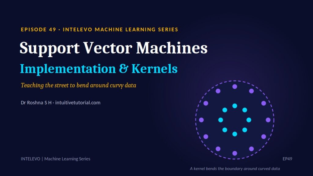
Imagine one class sitting inside a ring of the other class, like a bullseye target. The inner group clusters near the center. The outer group surrounds it on every side. Now try to draw a straight line that separates them.
You can’t. No matter how you rotate that line, it always cuts through one group or the other. A wide street cannot exist here either, because the outer group completely encloses the inner class. Consequently, the boundary itself needs to curve.
This scenario is not rare. Circular clusters, spirals, and nested groups show up constantly in real datasets — customer segments, image patterns, sensor readings. Therefore, a technique that only draws straight lines quickly hits a wall. Kernels solve this exact problem.
The Big Idea: The Kernel Trick
Here is the intuition. Picture your flat, two-dimensional data as a page lying on a table. Now imagine lifting the middle of that page upward, like pinching the center of a tablecloth and pulling it toward the ceiling. Once you view the lifted page from the side, a flat street can now separate what a circle on the original page could never separate.
That lift is the essence of the kernel trick. However, SVM never actually performs this lift in practice. Instead, it uses a shortcut called a kernel function to compute the effect of the lift, without ever touching the higher-dimensional space directly.
Mathematically, a kernel looks like this:
K(x, x′) = φ(x) · φ(x′)
In plain words, a kernel measures how similar two points are, as if the lift had already happened. You will never need to compute this by hand. Scikit-learn handles it instantly behind the scenes. The intuition matters far more than the formula: kernels give you the benefit of a curved boundary, without the cost of actually moving your data anywhere.
Meet the Three Kernels
Scikit-learn ships with several kernel options, but three cover almost every real-world case. Think of each one as a different kind of street.
| Kernel | Behavior | scikit-learn setting |
|---|---|---|
| Linear | A plain, straight street. Fast and easy to explain. | kernel='linear' |
| Polynomial | A street with gentle, predictable curves and bends. | kernel='poly' |
| RBF (Radial Basis Function) | A street that wraps around almost any shape at all. | kernel='rbf' |
The linear kernel works best when your classes already separate cleanly along a line. It trains fast, and its results are simple to interpret. Use it as a first check on any new dataset.
The polynomial kernel adds curvature in a controlled, predictable way. It fits well when you have a specific reason to expect polynomial-style interactions between features. That said, it needs careful validation, since it can overfit if the degree grows too high.
The RBF kernel handles almost any shape you throw at it. As a result, scikit-learn treats it as the default choice, and for good reason. When you are unsure what your data’s boundary looks like, start here.
A New Dial: Gamma
Once you move to a curved kernel like RBF, a second parameter enters the picture: gamma. Gamma decides how closely the boundary follows each individual point. Think of it as a dial for how snugly the street hugs the curb.
With low gamma, the street stays smooth and far-reaching. Even distant points influence its shape. This setting risks being too simple to capture real curves in your data.
With high gamma, the street becomes tight and wiggly. It hugs each nearby point closely, sometimes too closely. This setting risks memorizing the training data rather than learning a pattern that generalizes — a classic sign of overfitting.
C and Gamma, Working Together
C and gamma do not work in isolation. Instead, they combine to shape the entire decision boundary.
- Low C, low gamma produces a wide, smooth street. It stays simple and safe.
- Low C, high gamma produces a tolerant but wiggly boundary — an unusual mix.
- High C, low gamma produces a strict but smooth boundary, steady and dependable.
- High C, high gamma produces a strict, wiggly boundary. This combination overfits most easily, so use it with caution.
Once you see these four combinations side by side, tuning SVM stops feeling like guesswork. Instead, it becomes a matter of nudging two dials with a clear mental model of what each one does.
Let’s See It in Code
Theory only goes so far. Let’s implement all three kernels and compare them directly on a dataset that a straight line could never separate.
from sklearn.svm import SVC
from sklearn.datasets import make_circles
from sklearn.model_selection import train_test_split
from sklearn.preprocessing import StandardScaler

X, y = make_circles(n_samples=200, noise=0.1, factor=0.4)
X_train, X_test, y_train, y_test = train_test_split(X, y)

# Always scale before SVM — distances must be meaningful
scaler = StandardScaler()
X_train = scaler.fit_transform(X_train)
X_test = scaler.transform(X_test)

for k in ['linear', 'poly', 'rbf']:
    model = SVC(kernel=k, C=1.0, gamma='scale')
    model.fit(X_train, y_train)
    print(k, '→', model.score(X_test, y_test))
Let’s walk through this step by step. First, make_circles generates exactly the ring-shaped dataset we discussed earlier: one class nested inside another. Next, StandardScaler rescales every feature. This step is not optional. Since SVM measures distance between points, unscaled features distort the boundary for every kernel, not just the curved ones.
Notice that the scaler fits only on the training data, then transforms the test data separately. This order matters, because it prevents information from the test set leaking into training.
Finally, the loop trains all three kernels with identical settings for C and gamma, and prints each one’s accuracy. One short loop, therefore, gives you a direct, apples-to-apples comparison.
Reading the Output
Running the snippet above produces something like this:
linear → 0.54
poly   → 0.86
rbf    → 0.98
The linear kernel barely beats a coin flip. That result makes sense — a straight street simply cannot follow a circle. The polynomial kernel performs noticeably better. Meanwhile, the RBF kernel bends its boundary to match the ring shape almost perfectly, reaching 98 percent accuracy.
This single comparison tells the whole story. Choosing the right kernel often matters more than any other tuning decision you’ll make.
A few things worth trying on your own: change gamma='scale' to gamma=5 on the RBF model, then watch accuracy start to slip as the model overfits. Print model.n_support_ to see how many support vectors each kernel actually needed. Finally, plot the decision boundary for each kernel with matplotlib for a visual gut-check.
Tuning the Dials Automatically
Guessing C and gamma by hand wastes time, and it rarely finds the best combination. GridSearchCV solves this by testing many combinations automatically, then keeping whichever one generalizes best.
from sklearn.model_selection import GridSearchCV

params = {
    'C': [0.1, 1, 10],
    'gamma': [0.01, 0.1, 1],
}

search = GridSearchCV(
    SVC(kernel='rbf'), params, cv=5
)
search.fit(X_train, y_train)

print(search.best_params_)
Here, cv=5 means each combination runs through five different train-validation splits. This idea should feel familiar if you followed our earlier episode on cross-validation; the same principle now applies to picking hyperparameters instead of picking data.
Once search.fit finishes, search.best_params_ hands you the exact C and gamma combination that performed best on average. No more guesswork, and no more manual trial and error.
Choosing a Kernel: A Practical Guide
Use this quick reference the next time you start a new classification project:
- If your data looks separable by a line, start with linear. It trains fastest and stays easiest to explain.
- If the shape of your boundary is unknown, start with RBF. It offers the safest, most flexible default.
- If you have a strong, specific reason to expect polynomial interactions, try poly, but validate carefully.
- If you have many features but very few samples, such as text data, linear often already separates classes well.
As a general rule of thumb, scale your features first. Then default to RBF, and grid-search from there if accuracy needs a boost.
Common Pitfalls to Avoid
A handful of mistakes trip up most beginners, so watch for these directly.
Skipping StandardScaler ranks as the most common error. Since SVM measures distance, unscaled features silently distort every kernel’s results, often without any obvious warning sign.
Setting gamma too high causes the model to memorize training points instead of learning a general pattern. As a result, accuracy on new data drops even as training accuracy looks perfect.
Picking C and gamma by hand wastes time that GridSearchCV could spend more productively. It explores far more combinations than manual testing ever could.
Ignoring dataset size creates slowdowns later. Non-linear kernels train noticeably slower on very large datasets, so plan your training time accordingly.
Strengths and Trade-offs
Every technique comes with trade-offs, and kernel SVMs are no exception.
On the strengths side, a one-line change — kernel='rbf' — handles almost any boundary shape. You skip manual feature engineering entirely, since the kernel captures curves for you. SVM also stays memory-efficient, because it only stores the support vectors rather than the entire dataset.
On the trade-offs side, you now manage two dials instead of one. Training slows down on very large datasets. The resulting boundary also becomes harder to interpret than a simple straight line, and a high gamma can overfit if you leave it unchecked.
Weighing these trade-offs upfront saves you time later, especially on large or noisy datasets.
Five Things to Remember
Before you move on, keep these five points in mind:
- Kernels let SVM bend straight streets around curved data.
- Linear, polynomial, and RBF give you three tools for three different shapes.
- Gamma controls how tightly the boundary hugs the data.
- C and gamma together set the strictness and curviness of the final boundary.
- Always scale your features first, then let GridSearchCV pick both dials for you.
Watch the Full Video
This article covers the written version of Episode 49 from the Intelevo Machine Learning Series. For the complete walkthrough, including the visual explanations of the kernel trick and a live look at each decision boundary, watch the video on YouTube. Then, subscribe so you don’t miss what comes next.
In the next episode, EP50, we shift focus to Multi-class Classification Strategies — how SVM, originally built for just two classes, learns to tell many classes apart. See you there.
Enjoyed this article? Like the video, subscribe to Intelevo, and drop your questions or feedback in the comments — it genuinely helps this series reach more learners like you.