Stable diffusion models stand out for their ability to capture intricate data distributions while maintaining stability during training and inference. Unlike traditional approaches that may suffer from issues like mode collapse or vanishing gradients, stable diffusion models offer a robust solution for tasks ranging from image generation to data denoising.
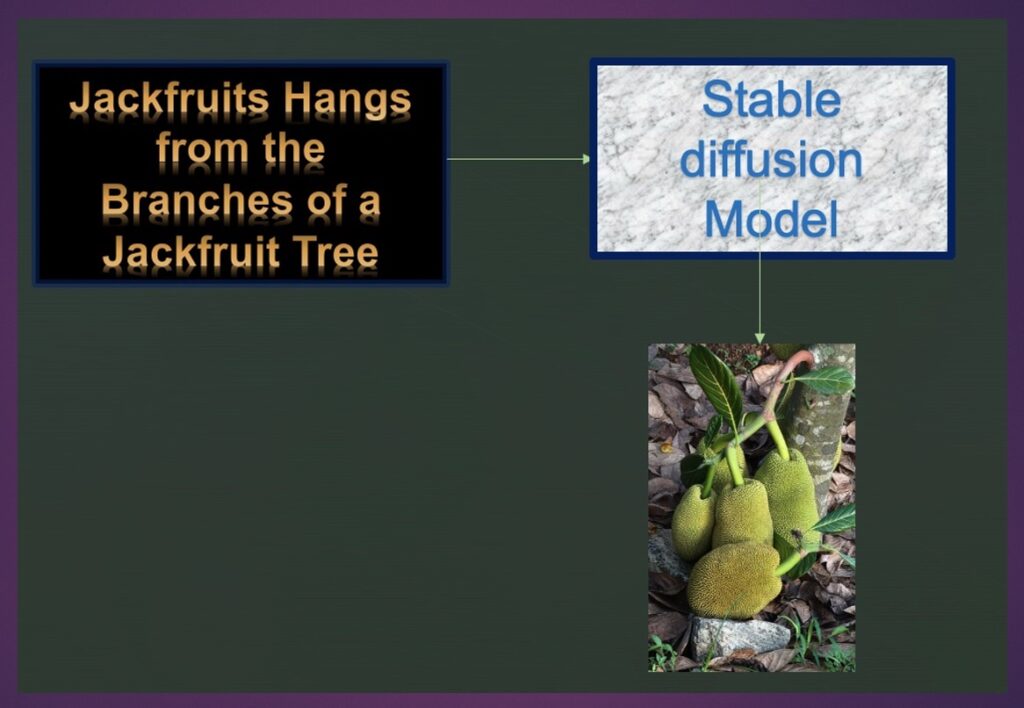
The title image depicting a text box with the phrase “jackfruits hang from the branches of a jackfruit tree” undergoing transformation through a stable diffusion model serves as a fitting visual representation of the intricate process underlying these advanced models.
Just as the text gradually evolves into an image, stable diffusion models employ controlled diffusion processes to transform simple input distributions into complex, high-dimensional data representations. This introductory schematic encapsulates the essence of stable diffusion models, which excel in tasks such as image generation, data denoising, and synthesis by progressively refining the input to produce realistic and diverse outputs. In this article, we will explore the principles, applications, and innovations driving the development of stable diffusion models in the realm of machine learning.
“Diffusion” in Stable Diffusion Models
In a stable diffusion model, “diffusion” signifies the process whereby the model gradually transforms an initial distribution (typically a simple and known distribution, such as Gaussian noise) into a target distribution (often the data distribution we want to model or generate samples from). This transformation occurs through a series of controlled steps or iterations.
The term “diffusion” originates from physics, where it describes the spread of particles or molecules from an area of high concentration to an area of low concentration. In machine learning, diffusion models utilize similar principles to guide the model towards generating realistic samples resembling the true data distribution.
The diffusion process in stable diffusion models typically involves iteratively transforming the input distribution by applying a series of diffusion steps. Each diffusion step introduces controlled noise or perturbations to the data, gradually spreading out the probability mass and bringing the distribution closer to the target distribution. This controlled spreading of the probability mass ensures that the model generates diverse and realistic samples while maintaining stability during training.
By decomposing the generation process into a sequence of diffusion steps, stable diffusion models offer several advantages, including improved training stability, better convergence properties, and enhanced interpretability. Moreover, the diffusion process allows the model to effectively capture complex data distributions across diverse domains, ranging from images and text to audio and beyond.
Overall, diffusion plays a central role in stable diffusion models by facilitating the gradual transformation of an initial distribution into a target distribution, enabling the generation of high-quality and diverse samples in machine learning tasks.
How diffusion works?
Initially, imagine a simple distribution, such as random noise, represented by a cluster of points. As the diffusion process unfolds, controlled perturbations are introduced gradually. These perturbations cause the points to spread out, resembling the diffusion of particles in a solution.
Over successive iterations, the distribution becomes increasingly diffuse, eventually converging towards the target distribution. This step-by-step transformation exemplifies the essence of diffusion in stable diffusion models, where controlled spreading of probability mass leads to the generation of realistic and diverse data samples
Components of a Stable Diffusion Model
A stable diffusion model comprises several key components, each playing a crucial role in its functioning. Let’s break down these components and provide Python code snippets along with explanations for each part.
1. Generator Architecture:
The generator is the core component of a stable diffusion model responsible for transforming random noise into meaningful data samples. It typically consists of neural network layers designed to learn the mapping from the input noise space to the target data distribution
Example:
import torch
from torch import nn

class Generator(nn.Module):
    def __init__(self, input_dim, output_dim):
        super(Generator, self).__init__()
        self.fc = nn.Linear(input_dim, 256)
        self.relu = nn.ReLU()
        self.out = nn.Linear(256, output_dim)

    def forward(self, x):
        x = self.relu(self.fc(x))
        x = self.out(x)
        return x
Explanation: In this example, we define a simple generator architecture using fully connected layers (linear) and activation functions (ReLU). The input dimension represents the size of the input noise space, while the output dimension corresponds to the dimensionality of the generated data samples.
2. Diffusion Process:
The diffusion process involves iteratively transforming the input noise into data samples by applying controlled perturbations. Each diffusion step gradually refines the noise distribution, bringing it closer to the target data distribution.
Example:
def diffusion_process(generator, input_noise, num_steps):
    for _ in range(num_steps):
        noise_diff = torch.randn_like(input_noise)
        generated_sample = generator(input_noise)
        input_noise += noise_diff * generated_sample
    return input_noise
Explanation: This code snippet demonstrates the diffusion process, where the input noise is iteratively refined by adding noise scaled by the output of the generator. By repeating this process for a specified number of steps, the input noise evolves into a sample resembling the target data distribution.
3. Loss Function
The loss function quantifies the discrepancy between the generated samples and the target data distribution. It guides the training process by minimizing this discrepancy, thereby encouraging the generator to produce more realistic samples
Example:
criterion = nn.MSELoss()
Explanation: Here, we define the Mean Squared Error (MSE) loss function, commonly used in stable diffusion models. This loss measures the squared difference between the generated samples and the target data samples.
4. Training Loop:
The training loop orchestrates the training process by iteratively updating the parameters of the generator to minimize the loss function.
Example:
optimizer = torch.optim.Adam(generator.parameters(), lr=learning_rate)

for epoch in range(num_epochs):
    optimizer.zero_grad()
    generated_samples = generator(input_noise)
    loss = criterion(generated_samples, target_data)
    loss.backward()
    optimizer.step()
Explanation: In this snippet, we define an Adam optimizer to update the parameters of the generator based on the computed gradients. Inside the training loop, we generate samples from the generator, compute the loss, perform backpropagation, and update the model parameters accordingly.
By understanding and implementing these components, one can construct and train stable diffusion models effectively for various machine learning tasks, such as image generation and data synthesis
Applications of Stable Diffusion Models
Stable diffusion models find applications across various domains in machine learning, offering robust solutions for tasks such as image generation, data denoising, and image inpainting. Let’s explore some concrete use cases along with examples, Python code snippets, and explanations.
1. Image Generation:
One of the primary applications of stable diffusion models is in generating high-quality and diverse images. Let’s consider the task of generating realistic images of handwritten digits using the MNIST dataset.
Example:
import torch
from torchvision.utils import save_image
from torchvision.utils import make_grid
from torchvision.datasets import MNIST
from torch.utils.data import DataLoader
from torch import nn

# Define a stable diffusion model architecture
class Generator(nn.Module):
    def __init__(self, input_dim, output_dim):
        super(Generator, self).__init__()
        # Define your architecture here (e.g., using convolutional layers)

    def forward(self, x):
        # Forward pass logic
        return generated_image

# Load MNIST dataset
dataset = MNIST(root='data/', train=True, transform=transform, download=True)
dataloader = DataLoader(dataset, batch_size=batch_size, shuffle=True)

# Instantiate and train the stable diffusion model
generator = Generator(input_dim, output_dim)
criterion = nn.MSELoss()
optimizer = torch.optim.Adam(generator.parameters(), lr=learning_rate)

for epoch in range(num_epochs):
    for batch_idx, (real_images, _) in enumerate(dataloader):
        # Generate fake images
        fake_images = generator(input_noise)

        # Compute loss
        loss = criterion(fake_images, real_images)

        # Backpropagation
        optimizer.zero_grad()
        loss.backward()
        optimizer.step()

# Generate samples from the trained model
with torch.no_grad():
    generated_samples = generator(sample_noise)

# Visualize generated samples
save_image(make_grid(generated_samples), 'generated_samples.png')
Explanation: In this example, we define a simple generator model architecture for generating images of handwritten digits from the MNIST dataset. We then train the generator using a stable diffusion approach, where the generator gradually transforms random noise into realistic images resembling the digits in the MNIST dataset. Finally, we generate samples from the trained model and visualize them to assess the quality of the generated images.
Note:
You can download the MNIST dataset directly using Python code. Here’s a code snippet using the popular torchvision library
import torchvision.datasets as datasets

# Download MNIST train and test datasets
train_dataset = datasets.MNIST(root='.', train=True, download=True)
test_dataset = datasets.MNIST(root='.', train=False, download=True)
This code will download the MNIST train and test datasets to the current directory ('.'). If you want to specify a different directory, you can change the root parameter accordingly.
Make sure you have the torchvision library installed. If not, you can install it using pip:
pip install torchvision
Once you run this code snippet, you’ll have the MNIST dataset downloaded and ready to use in this environment.
2. Data Denoising
Stable diffusion models can also be used for denoising noisy data, such as images corrupted by random noise or artifacts.
Example:
import torch
from torchvision.utils import save_image
from torchvision.datasets import CIFAR10
from torch.utils.data import DataLoader
from torch import nn

# Define a stable diffusion model architecture for denoising
class Denoiser(nn.Module):
    def __init__(self, input_dim, output_dim):
        super(Denoiser, self).__init__()
        # Define your architecture here (e.g., using convolutional layers)

    def forward(self, x):
        # Forward pass logic
        return denoised_image

# Load CIFAR-10 dataset with added noise
dataset = CIFAR10(root='data/', train=True, transform=transform, download=True)
dataloader = DataLoader(dataset, batch_size=batch_size, shuffle=True)

# Instantiate and train the denoiser model
denoiser = Denoiser(input_dim, output_dim)
criterion = nn.MSELoss()
optimizer = torch.optim.Adam(denoiser.parameters(), lr=learning_rate)

for epoch in range(num_epochs):
    for batch_idx, (noisy_images, _) in enumerate(dataloader):
        # Denoise noisy images
        denoised_images = denoiser(noisy_images)

        # Compute loss
        loss = criterion(denoised_images, clean_images)

        # Backpropagation
        optimizer.zero_grad()
        loss.backward()
        optimizer.step()

# Visualize denoised images
save_image(make_grid(denoised_images), 'denoised_images.png')
Explanation: In this example, we demonstrate how stable diffusion models can be used for denoising noisy images from the CIFAR-10 dataset. We define a denoiser model architecture and train it to transform noisy images into clean versions. The stable diffusion approach allows the denoiser to gradually remove noise and artifacts from the input images, resulting in visually pleasing and high-quality denoised images. Finally, we visualize the denoised images to evaluate the performance of the trained denoiser model.
Note:
You can download the CIFAR-10 dataset directly using Python code. Here’s a code snippet using the torchvision library:
import torchvision.datasets as datasets

# Download CIFAR-10 train and test datasets
train_dataset = datasets.CIFAR10(root='.', train=True, download=True)
test_dataset = datasets.CIFAR10(root='.', train=False, download=True)
This code will download the CIFAR-10 train and test datasets to the current directory ('.'). If you want to specify a different directory, you can change the root parameter accordingly.
Just like with the MNIST dataset, make sure you have the torchvision library installed. If not, you can install it using pip:
pip install torchvision
After running this code snippet, you’ll have the CIFAR-10 dataset downloaded and ready to use in this environment.
These examples showcase the versatility and effectiveness of stable diffusion models in various machine learning tasks, including image generation and data denoising. By leveraging controlled diffusion processes, these models offer robust solutions for generating realistic samples and enhancing the quality of noisy data.
Endnote
Your feedback is valuable. Let us know your thoughts to enhance future articles.
If you are aspirant of data science job roles, we have compiled frequently asked interview questions for you
If you would like to explore more in machine learning, do visit machine learning fundamentals
Subscribe to this website for email notifications