Introduction
TinyML is the field which involves deployment of machine learning models into resource constrained devices such as micro-controllers. Such devices called edge devices often have few Kilobytes of RAM and flash memory but consumes power in milli-watts range. This feature makes the technology an ideal choice for remote sensing applications, weather stations, tiny gadgets etc.
The field of TinyML is evolving by solving various real-life problems. Consider a smart watch measuring the number of steps you have taken every day. By adding reminders at occasions needed will help you stay fit and healthy. Creative applications of such a category often require applying deep learning to create models which can do predictions on new data. For example, a face recognition system can be part of a door locking and unlocking mechanism. Also it can monitor employee attendance by observing their check in and checkout time.
Developers Train of such machine learning models often in desktop PCs or cloud computing infrastructure. The raw data used (e.g. images or audios) often has higher resolution such as 32 bit floating point. The machine learning modeling achieves precision and operates on computers with such precision and operating systems.
Low-power IoT devices often run on micro-controllers without operating systems, limited software, and hardware. Moreover the resolution of datatypes is often 8-bit or 16-bit floating point numbers. Machine learning models trained on high-end PCs need to scale down so that they can run on such micro-controllers and quantize input data, reducing the amount of levels a signal can represent.
What we will learn in this tutorial
In this tutorial, we will create a simple deep learning model that approximates the trigonometric sine function. We will see how to train such a model, and convert it using TinyML concepts so that it is deployable to microcontrollers. First let us take a look at the data modeling/training part. A Google Colab corresponding to the Jupyter Notebook is provided here. Now let me walk you through the individual parts of the code. First let us import the required libraries.
Import Libraries
import math
import random
import pathlib
import numpy as np
import tensorflow as tf
from keras.layers import Dense
import matplotlib.pyplot as plt
from keras.models import Sequential
from tensorflow.saved_model import save
The step is to define the constant values we will be using in this program at a single place. This will help us with code modification and experimentation easier. We only need to change the code at a single place and rerun the code to see the changes.
Parameter Settings
NUM_DATA_POINTS = 1000
LEARNING_RATE = 0.001
BATCH_SIZE = 128
EPOCHS = 200
NUM_TEST_DATA_POINTS = 50
SEED = 1337
Along with this we will also set a random seed so that we will get some consistency when we call functions involving some randomness. We will create some folders where we can save the original deep learning models as well as the TinyML converted model.
np.random.seed(SEED)
tf.random.set_seed(SEED)
Generating Dataset
To train a machine learning model, we need to have both features and labels. In our case, the function we are trying to approximate is a simple sine function. We will use builtin sine function in the numpy library to generate X, y pairs of training data.
def generate_dataset(num_data_points):
  X = np.random.uniform(low=0, high=2*math.pi, size=num_data_points)
  np.random.shuffle(X)
  y = np.sin(X)
  return X, y
X, y = generate_dataset(NUM_DATA_POINTS)
Define Model Architecture
To approximate the sine function using neural networks, we can use dense blocks. Although there are various types of neural network blocks available such as convolutional blocks, dense blocks, LSTM etc. our application requires only dense blocks to serve the purpose. The following code shows a function which creates a deep neural network and returns it. Please note that the number of units in the last layer is one. This is because we are predicting only a scalar value which is equivalent to the sine transformation to the input value.
def create_dnn_model():
    model = Sequential()
    model.add(Dense(32, input_shape = (1,), activation='relu'))
    model.add(Dense(64, activation='relu'))
    model.add(Dense(16, activation='relu'))
    model.add(Dense(1))
    return model
model = create_dnn_model()
By calling the model.summary() function, we will get a snapshot of the individual layers, number of units in each layer and number of parameters in each layer.
model.summary()
Model: "sequential"
_________________________________________________________________
 Layer (type)                Output Shape              Param #
=================================================================
 dense (Dense)               (None, 32)                64

 dense_1 (Dense)             (None, 64)                2112

 dense_2 (Dense)             (None, 16)                1040

 dense_3 (Dense)             (None, 1)                 17

=================================================================
Total params: 3233 (12.63 KB)
Trainable params: 3233 (12.63 KB)
Non-trainable params: 0 (0.00 Byte)
_________________________________________________________________
The next step would be compiling the model by specifying the optimizer to use and the loss metrics.
model.compile(optimizer='rmsprop', loss='mse', metrics=['mae'])
Now we will train the model by calling the model.fit() function. This function takes X and y pair values, batch size, epochs (the number of iterations for training), and the validation split percentage as inputs. The validation split determines the percentage of the total data to use for training the model and evaluating its performance after each iteration.
history = model.fit(X,
                    y,
                    batch_size=BATCH_SIZE,
                    epochs=EPOCHS,
                    validation_split=0.3)
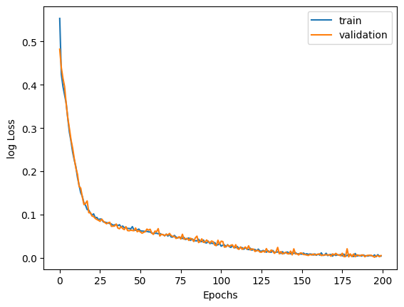
The history variable here contains the change of metrics after each iteration. The following function and plot shows how to compute and plot the train and validation loss curves using neat graphs.
def plot_history(history):
    plt.plot(history.history["loss"])
    plt.plot(history.history["val_loss"])
    plt.xlabel("Epochs")
    plt.ylabel("log Loss")
    plt.legend(["train", "validation"], loc="upper right")
    plt.show()
plot_history(history)
Prediction on Test Data
To double check to see if our neural network has learned to approximate sine function, we can again synthesize X, y pairs of data using random functions and numpy sine function. The model predicts the output to match both values with the same inputs.. Now lets visualise the results to how closely they match with each other.
X_test = np.random.uniform(low=0, high=2*math.pi, size=NUM_TEST_DATA_POINTS)
y_test = np.sin(X_test)
y_pred = model.predict(X_test)

plt.scatter(X_test, y_test, label="actual")
plt.scatter(X_test, y_pred, label="predicted")
plt.legend()
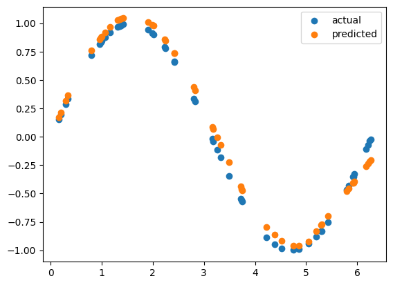
The above scatter plot shows the actual sine computed values on test data and values predicted by our model. As you can see both of them are overlapping nearly closely. This means our neural network model has learned to approximate the sine function fairly closely.
We have now saved the trained model, which is working fine, to a directory created earlier.
Conversion to TensorFlow Lite Model
In order to convert a given TensorFlow model to TinlyML model, we will be relying on the same TensorFlow library. To do that, we will load the model from the saved directory, initialize a TFLite converted object and save the converted file with an extension “.tflite”. The next line prints the file size in Kilobytes. The model needs to be small enough so that it can convert to a header file and load into micro-controller boards like Arduino.
export_dir = "saved_TF_model"
save(model, export_dir)

converter = tf.lite.TFLiteConverter.from_saved_model(export_dir)
tflite_model = converter.convert()

tflite_model_file = pathlib.Path("./model/model.tflite")
model_size_kb = tflite_model_file.write_bytes(tflite_model) / 1024
print("Size of TensorFlow Lite Model: {} KB:".format(model_size_kb))
Prediction using TFLite Model created
We can equivalently load the TFLite model and test on sample inputs within the python environment itself to see if it is working. The following code block shows that. We can check output for known inputs to see if it is working. The following code block shows how to do that.
sine_model = tf.lite.Interpreter('./model/model.tflite')

# Allocate memory for each model
sine_model.allocate_tensors()

# Get indexes of the input and output tensors
sine_model_input_index = sine_model.get_input_details()[0]["index"]
sine_model_output_index = sine_model.get_output_details()[0]["index"]

x = np.pi/2
x_value_tensor = tf.convert_to_tensor([[x]], dtype=np.float32)
sine_model.set_tensor(sine_model_input_index, x_value_tensor)

# Run inference
sine_model.invoke()

y_pred = sine_model.get_tensor(sine_model_output_index)[0][0]

print(f'x: {x:.4f}, y_pred: {y_pred:.4f}, y_actual: {np.sin(x):.4f}')

# Output x: 1.5708, y_pred: 1.0515, y_actual: 1.0000
Generate TFLite Micro Header File
To convert a given TFLite model to a header file we need command line tools such as xxd and sed. Since we are using Google Colab which is a virtual Linux machine, we need to install these tools before using it. The following command installs these command line tools.
!apt-get update && apt-get -qq install xxd
To convert the TFLite model to headerfile, we can use the following Linux commands.
MODEL_TFLITE = "./model/model.tflite"
MODEL_TFLITE_MICRO = "./model/model.h"
!xxd -i {MODEL_TFLITE} > {MODEL_TFLITE_MICRO}
REPLACE_TEXT = MODEL_TFLITE.replace('/', '_').replace('.', '_')
!sed -i 's/'{REPLACE_TEXT}'/g_model/g' {MODEL_TFLITE_MICRO}
This will save the header file with a name “model.h”.
Deployment to Arduino Nano BLE Sense
Many TinyML supported boards such as Arduino Nano BLE Sense, ESP32, SparkFunEdge, etc., are available in the market. In this tutorial, we will use Arduino Nano BLE Sense for the purpose of demonstration. In the Arduino IDE itself, we need to connect the device to the development PC via USB cable and verify if it detects in the serial port.
Once we connect and detect the device, we can write Arduino code to load the model header file, associated code, and start inference. The following code blocks show how to do that.
#include "model.h"
#include <arm_math.h>
#include <TensorFlowLite.h>
#include <tensorflow/lite/micro/all_ops_resolver.h>
#include <tensorflow/lite/micro/micro_interpreter.h>
#include <tensorflow/lite/micro/micro_log.h>
#include <tensorflow/lite/micro/system_setup.h>
#include <tensorflow/lite/schema/schema_generated.h>

namespace tflite
{
    namespace ops
    {
        namespace micro
        {

            TfLiteRegistration *Register_FULLY_CONNECTED();
        }
    }
}

namespace
{
    const tflite::Model *model = nullptr;
    tflite::MicroInterpreter *interpreter = nullptr;
    TfLiteTensor *model_input = nullptr;
    TfLiteTensor *model_output = nullptr;

    constexpr int kTensorArenaSize = 2 * 2048;
    uint8_t tensor_arena[kTensorArenaSize];

    float sinFrequency = 1; // Default frequency
    int numSamples = 1000;  // Default number of samples
}

void setup()
{
    Serial.begin(9600);
    while (!Serial)
    {
    };

    // initialize digital pin LED_BUILTIN as an output.
    pinMode(LED_BUILTIN, OUTPUT);

    model = tflite::GetModel(g_model);
    if (model->version() != TFLITE_SCHEMA_VERSION)
    {
        Serial.println("Schema mismatch");

        return;
    }
    // Pull in only the operation implementations we need.
    tflite::AllOpsResolver tflOpsResolver;

    // Build an interpreter to run the model with.
    static tflite::MicroInterpreter static_interpreter(
        model, tflOpsResolver, tensor_arena, kTensorArenaSize);
    interpreter = &static_interpreter;
    // Allocate memory from the tensor_arena for the model's tensors.
    TfLiteStatus allocate_status = interpreter->AllocateTensors();
    if (allocate_status != kTfLiteOk)
    {
        Serial.println("AllocateTensors() failed");
        return;
    }

    model_input = interpreter->input(0);
    model_output = interpreter->output(0);
}

void loop()
{

    for (int i = 0; i < numSamples; i++)
    {

        float x = 2 * PI * sinFrequency * i / numSamples;

        // Library Implementation of Sine Function
        // float y_pred = sin(x);

        // ML Approximation of Sine Function
        model_input->data.f[0] = x;

        TfLiteStatus invoke_status = interpreter->Invoke();
        if (invoke_status != kTfLiteOk)
        {
            Serial.println("Invoke failed");
            return;
        }

        float y_pred = model_output->data.f[0];

        Serial.println(y_pred);

        int ledState = y_pred * 255;
        analogWrite(LED_BUILTIN, ledState);
    }
}
Loading Header Files
We can include the header files using #include command. Here we will be including the model.h and tensorflow lite micro library. The next step is to add namespace for various learning blocks we need to add. In our case we have only used dense blocks hence we need to add namespace for FULLY_CONNECTED blocks only.
The next step is to define pointers for loading the model, model input and model output. We have to define a Tensor Arena Size as well. It is advisable to allocate enough space for this depending upon the size of data you need to process.
The rest of the program mainly consists of a setup function and loop functionThe board will execute the setup function only once and can use it for initializing various operators or classes.. Here we will be using the same of initializing the serial port, setting the output mode of builtin led, and loading the model from the header file.
Additionally we will be importing all the learning or functional blocks, initializing the interpreter, creating variables for model input and output.
Inside the void loop function we will simply create input values, pass those to the model input variable, invoke the interpreter, fetch the model output and print it. We can use the model predicted values for setting up builtin LED brightness. This will adjust the builtin LED’s brightness in a smooth sine wave like fashion.
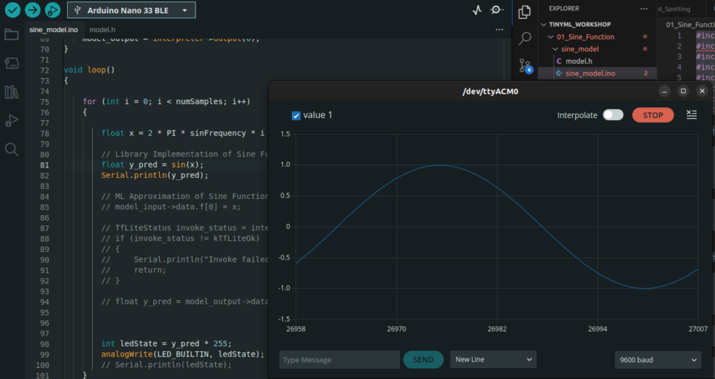
Flashing the Program
Finally we are ready to flash the program to the target device.
Pressing the compile and flash button in the Arduino IDE accomplishes this. After this step, you can observe the process flashing the code to the target device. If we open the serial plotter (please see the figure below), we will be able to see the sine wave graphs plotted and change in LED brightness according to the sine wave frequency.