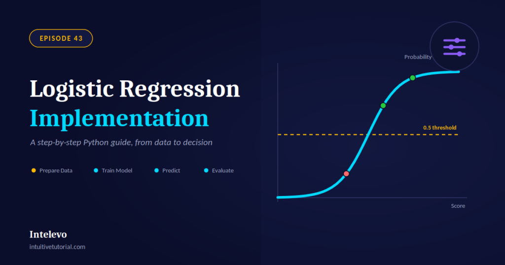
You already understand logistic regression, even if you have never written a single line of code for it. In our last episode, we compared it to a spam-o-meter dial. A score goes in, a probability comes out, and a threshold turns that probability into a clear decision. Today, we turn that idea into working Python code.
This article follows Episode 43 of the Intelevo YouTube series, where we build a complete logistic regression classifier from scratch. If you prefer to watch and follow along, the video walks through every line of code shown here. If you prefer to read at your own pace, this article covers the same ground in detail.
By the end, you will know how to prepare data, train a model, read its predictions, and check whether you can trust it. Let’s get started.
What You Will Build Today
Logistic regression solves one specific problem well: it answers yes-or-no questions using data. Will this email land in the spam folder? Will this transaction turn out fraudulent? Will this student pass the exam? Each of these questions has exactly two possible answers, and logistic regression handles that shape of problem better than almost any other beginner-friendly algorithm.
Our roadmap has three clear stages. First, we prepare a simple dataset. Next, we train the model and ask it for probabilities. Finally, we turn those probabilities into decisions and check how good those decisions really are. Every stage builds on the one before it, so nothing here requires advanced math or prior modeling experience.
Meet the Dataset
To keep things intuitive, we will use one input and one output. The input is hours studied for an exam. The output is whether the student passed, labeled as 1, or failed, labeled as 0. This mirrors the spam-versus-not-spam shape from our previous episode, just with new labels.
| Hours Studied | Result |
|---|---|
| 1.0 | Fail (0) |
| 2.5 | Fail (0) |
| 4.0 | Pass (1) |
| 5.5 | Pass (1) |
| 7.0 | Pass (1) |
Notice the pattern already forming in this small table. More hours generally lead to a pass. That relationship is exactly what our model will learn on its own, without us telling it the rule directly. This same approach also scales up easily. Swap in three hundred features instead of one, and the code below still works without any structural changes.
Step 1: Prepare the Data
Every machine learning project starts with clean, well-organized data. Here, we load our dataset with pandas and split it into training and test sets using scikit-learn.
import pandas as pd
from sklearn.model_selection import train_test_split

df = pd.read_csv("exam_scores.csv")
X = df[["hours_studied"]]
y = df["passed"]

X_train, X_test, y_train, y_test = train_test_split(
    X, y, test_size=0.2, random_state=42)
First, we import pandas to handle our data and train_test_split to divide it. Then, we load the CSV file into a dataframe. After that, we separate the input, X, from the answer, y. Finally, we split off 20 percent of the data as a test set.
Why bother with a split at all? Consider this: training and testing on the exact same data resembles grading a student on questions they have already seen the answers to. The held-out 20 percent acts as a genuine surprise quiz. It reveals whether the model actually learned the underlying pattern, or simply memorized the training examples.
Step 2: Train the Dial
With clean data in hand, training takes surprisingly little code.
from sklearn.linear_model import LogisticRegression

model = LogisticRegression()
model.fit(X_train, y_train)
Three lines complete the entire training step. So, what happens inside .fit()? Behind the scenes, scikit-learn tries many possible curves. It adjusts the dial until predictions align closely with the real pass-or-fail answers in the training set. Before training, the dial sits uncalibrated. Afterward, it knows roughly how many study hours reliably tip the scale toward a pass.
Notably, you never write the curve-fitting math by hand. Instead, scikit-learn searches for the best-fitting curve automatically, which is exactly why logistic regression remains such an approachable algorithm for beginners.
Step 3: Ask the Dial for a Probability
Once trained, the model can estimate a probability for any new student.
probs = model.predict_proba(X_test)
print(probs[:3])
# [[0.81, 0.19],
#  [0.27, 0.73],
#  [0.05, 0.95]]
Each row in this output holds two numbers: the probability of failing and the probability of passing. Take the first row as an example. It shows a 19 percent chance of passing, so the dial leans toward “fail.” Meanwhile, the third row shows a 95 percent chance of passing, meaning the dial leans hard toward “pass.”
This step matters because it exposes the model’s confidence, not just its final answer. A probability of 51 percent and a probability of 99 percent both round to “pass,” yet they represent very different levels of certainty. Keeping that nuance visible often proves useful in real projects, especially when a wrong prediction carries a real cost.
Step 4: Cross the Threshold with predict()
Probabilities are informative, but sooner or later, a project needs a firm decision. That is exactly what .predict() provides.
preds = model.predict(X_test)
print(preds[:3])
# [0, 1, 1]
The rule behind .predict() stays simple throughout. If the probability reaches 0.5 or higher, the predicted class becomes 1, meaning pass. If it falls below 0.5, the predicted class becomes 0, meaning fail. This 0.5 line works exactly like the velvet rope from our spam-o-meter analogy: one consistent rule, applied identically to every single prediction.
Understanding What the Model Learned
It helps to peek inside the trained model and see what it actually learned.
print("Coefficient:", model.coef_)
print("Intercept:", model.intercept_)
# Coefficient: [1.4]
# Intercept:   [-5.2]
In plain terms, a positive coefficient means additional study hours push the dial toward a pass. Furthermore, a larger coefficient means each extra hour swings the dial harder. The intercept simply sets where the dial starts when hours studied equals zero.
One small formula sits behind this idea:
odds = coefficient × hours + intercept
The sigmoid function then squashes that raw number into a clean probability between 0 and 1. You do not need to solve this equation by hand, since scikit-learn already handled it during training. What matters most for intuition is the direction of the coefficient: a positive value consistently means “more likely,” while a negative value means “less likely.”
Evaluating the Model: Accuracy and the Confusion Matrix
Training a model is only half the job. Checking its performance honestly matters just as much.
from sklearn.metrics import accuracy_score, confusion_matrix

accuracy_score(y_test, preds)
confusion_matrix(y_test, preds)
Accuracy gives one simple number: the fraction of students the model classified correctly. However, a single number can hide important details. That is where the confusion matrix helps. It breaks results down into four categories: correct passes, correct fails, and the two distinct ways a prediction can go wrong.
| Predicted: Fail | Predicted: Pass | |
|---|---|---|
| Actual: Fail | 9 | 1 |
| Actual: Pass | 2 | 13 |
In this example, the model correctly classifies 22 out of 25 students, which works out to 88 percent accuracy. That single figure looks impressive on its own, but the next section explains why it should never stand alone.
Beyond Accuracy: Precision and Recall
This caution connects directly back to our earlier episode on imbalanced datasets. Imagine a scenario where 95 out of 100 students genuinely pass. A lazy model that predicts “pass” for absolutely everyone would score 95 percent accuracy, despite learning nothing meaningful at all. Clearly, accuracy alone can mislead.
from sklearn.metrics import precision_score, recall_score

precision_score(y_test, preds)
recall_score(y_test, preds)
Precision answers one specific question: of the students predicted to pass, how many actually passed? Recall answers a different question: of the students who genuinely passed, how many did the model correctly catch? As a rule of thumb, watch recall closely when missing a true positive worries you. On the other hand, watch precision closely when false alarms carry a real cost. Either way, always check class balance before trusting a single accuracy figure.
Four Common Mistakes to Avoid
Before shipping a logistic regression model of your own, keep these four pitfalls in mind.
Unscaled features. Mixing a feature like hours studied with a feature like annual income causes trouble, unless you scale both first. Without scaling, the larger numbers dominate the dial unfairly. Consequently, the model may weigh the wrong signal too heavily.
Ignoring class imbalance. A rare positive class needs precision, recall, or resampling techniques, not accuracy alone. Otherwise, the model can look impressive on paper while performing poorly where it actually matters.
Piling on too many features. Adding unrelated inputs invites overfitting, where the model memorizes training data instead of learning a genuine, generalizable pattern.
Treating 0.5 as fixed. The threshold does not have to sit at 0.5. In fact, moving it makes sense whenever false positives and false negatives carry different real-world costs.
The Complete Pipeline in Ten Lines
Zooming all the way out, here is the entire workflow in one place.
from sklearn.linear_model import LogisticRegression
from sklearn.model_selection import train_test_split
from sklearn.metrics import accuracy_score

X_train, X_test, y_train, y_test = train_test_split(X, y, test_size=0.2)

model = LogisticRegression().fit(X_train, y_train)
preds = model.predict(X_test)

print("Accuracy:", accuracy_score(y_test, preds))
Split, train, predict, check. That short sequence describes a complete, working classifier in roughly ten lines of Python. If you remember nothing else from this guide, remember this block. It condenses the whole idea into a form you can reuse on almost any binary classification problem.
Key Takeaways
Let’s bring everything together into four core ideas.
First, logistic regression is one dial, one idea: a raw score bends into a probability. Second, four scikit-learn calls handle the heavy lifting: split, fit, predict, and score. Third, coefficients simply reveal which direction, and how strongly, the dial swings. Fourth, accuracy marks only a starting point; precision and recall complete the fuller picture.
If you walked into this guide feeling unsure about logistic regression, it should feel genuinely approachable by now. Underneath all the terminology, the idea really is this simple.
Frequently Asked Questions
Is logistic regression used for regression or classification? Despite its name, logistic regression solves classification problems, not regression problems. It predicts categories, such as pass or fail, rather than continuous numbers.
Do I need to scale my features before training? Yes, in most real projects. Scaling prevents features with larger numeric ranges from dominating the model unfairly, which leads to more balanced, trustworthy coefficients.
Can logistic regression handle more than two classes? Yes. Scikit-learn extends logistic regression to multiple classes automatically, using a technique called multinomial logistic regression, so the same core idea scales beyond simple yes-or-no problems.
What is a good accuracy score for a beginner project? It depends entirely on the dataset and the class balance. A model can post high accuracy and still perform poorly on the class that matters most, so always check precision and recall alongside accuracy.
Why did my model’s coefficient come out negative? A negative coefficient simply means that feature pushes predictions toward the opposite class as it increases. It is not an error; it is useful information about the direction of the relationship.
Watch the Full Video Walkthrough
This article pairs directly with Episode 43 on the Intelevo YouTube channel, where every code block above gets explained line by line, alongside visual breakdowns of the sigmoid curve, the decision threshold, and the confusion matrix. If this guide helped clarify logistic regression for you, the video adds even more context and worked examples.
Up next, Episode 44 introduces K-Nearest Neighbors, a completely different approach to classification that works by asking your closest data neighbors for their opinion. Subscribe to the channel so you do not miss it, and drop a comment on the video with any questions about today’s implementation. Your feedback genuinely shapes future episodes.
This article accompanies the Intelevo Machine Learning series at intuitivetutorial.com. Explore earlier episodes to review classification fundamentals, imbalanced datasets, and the theory behind logistic regression.