Gradient Boosting Machines power a huge share of the models that win Kaggle competitions, rank your search results, and price your insurance policy. Yet most explanations jump straight into loss functions and partial derivatives. This guide skips that route. Instead, it builds the idea from a single, simple picture: an archer correcting each shot based on the last one’s miss.
By the end, you’ll understand exactly how Gradient Boosting Machines learn, why they work so well on real-world data, and how to train one yourself in a few lines of Python. This article is the companion piece to Episode 64 of the Intelevo Machine Learning Series. Watch the full video first if you’d like the visual walkthrough, then use this article to review the concepts and revisit the code.
A Quick Recap: From AdaBoost to Gradient Boosting
In the last episode, we covered AdaBoost. AdaBoost trains a chain of very simple learners, called stumps, one after another. After each round, it looks at which points the model got wrong. Then, it increases their weight. As a result, the next learner pays closer attention to those hard cases.
That approach works well. However, it has a subtle limitation. Reweighting a point tells the next learner “this one matters more.” It never tells the learner exactly how wrong the previous guess was. In other words, AdaBoost adjusts attention, not accuracy.
This is exactly the gap Gradient Boosting Machines close. Instead of reweighting data points, GBM aims directly at the size of the mistake. That single shift changes everything about how the model learns, so let’s unpack it properly.
The Big Idea: The Archer Who Aims at the Miss
Picture an archer shooting arrow after arrow at the same target. With a single shot, there’s no second chance. The arrow either lands close to the bullseye, or it doesn’t. Nothing corrects it afterward.
Now, picture a different archer. This one shoots, checks exactly how far the arrow landed from the bullseye, and adjusts the next shot accordingly. Each new shot closes the gap a little more than the last one did. Round after round, the shots cluster closer to the center.
That second archer is Gradient Boosting Machines in a nutshell. Every new “shot,” or tree, gets trained to correct exactly what the previous shots got wrong. Nothing gets reweighted. Instead, the model chases the leftover error directly, one small correction at a time.
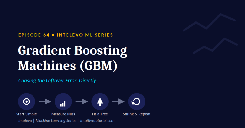
This habit of aiming at the miss has a name: Gradient Boosting. GBM stands for Gradient Boosting Machine, and the entire algorithm reduces to three repeating moves:
- Start simple. Begin with one plain guess for every row of data.
- Measure and fit the miss. Find out how far off that guess is, then train a small tree to predict that exact gap.
- Add the correction in, and repeat. Add the new tree’s prediction back in, a little at a time, and go again on whatever’s still missed.
That’s the whole algorithm. Now, let’s slow down and walk through each step in detail.
How Gradient Boosting Machines Work, Step by Step
Step 1: Start With One Plain Guess
Before Gradient Boosting Machines train a single tree, they make the simplest prediction possible: the average of every target value in the training data. Suppose you’re predicting house prices. The very first prediction is just the average house price, applied to every single row.
This might sound too simple to matter. However, that’s exactly the point. This baseline guess only needs to beat “no model at all.” Every tree that follows simply adds a correction on top of this one number.
Step 2: Measure the Miss
Next, the model checks how far off that baseline guess really is. This gap has a name: the residual. The formula is refreshingly simple:
residual = actual value − current prediction
Suppose a house actually sold for ₹50 lakhs, but the baseline guess said ₹42 lakhs for every house. The residual for that house is ₹8 lakhs. Here’s the twist that separates Gradient Boosting Machines from anything we’ve seen before: that residual, not the house price, becomes the new target to predict.
Step 3: Fit a Tree to the Miss, Not the Original Target
Now, the model trains a small decision tree. Crucially, it doesn’t train this tree on house prices. It trains it on the residuals from Step 2. The tree’s only job is to predict how wrong the previous guess was, for each row.
Why bother with this indirect approach? Consider a tree trained to predict the price directly. It has to explain the entire pattern at once. A tree trained on the residual only has to explain what’s still wrong. That’s a much smaller, more manageable job, and it gets easier and easier with each additional round.
Step 4: Add the Correction In, But Only a Little
Once the new tree produces its correction, the model doesn’t add all of it back in immediately. Instead, it shrinks the correction using a small multiplier. The update rule looks like this:
new prediction = old prediction + (learning_rate × tree's correction)
Think back to the archer. Trusting one shot’s correction completely risks overshooting the target. So, Gradient Boosting Machines shrink each tree’s contribution using a hyperparameter called learning_rate, typically somewhere between 0.01 and 0.3.
Smaller learning rates make the model learn more cautiously. Consequently, they need more rounds to converge. In exchange, they usually produce a steadier, more reliable path toward accurate predictions.
Step 5: Repeat, Round After Round
The model then simply repeats Steps 2 through 4. Round one typically learns the big, obvious pattern in the data. Round two fixes whatever round one missed. Round three chases what’s still stubborn. This continues until the model reaches a chosen number of rounds, called n_estimators.
Each round nudges the total prediction a little closer to the truth. In fact, this process resembles walking downhill toward zero error, one small step at a time. That “walking downhill” image is exactly where the word gradient comes from. Every new tree points in the direction that reduces the error the most, and the model keeps stepping in that direction until it runs out of rounds or the error stops shrinking meaningfully.
AdaBoost vs Gradient Boosting: Side by Side
Because both algorithms build a chain of learners, they can look similar at first glance. However, the mechanics underneath differ significantly. This comparison makes the distinction concrete.
| Aspect | AdaBoost | Gradient Boosting Machines |
|---|---|---|
| What gets adjusted | Sample weights (attention) | Residual errors (the gap itself) |
| Correction target | Same labels, reweighted | The leftover error, directly |
| Base learner | Very shallow stumps (depth 1) | Slightly deeper trees (depth 3–8) |
| Combine method | Weighted vote (by accuracy) | Weighted sum (learning rate × trees) |
| Sensitivity to outliers | High — weights can explode | Moderate — tunable via loss and shrinkage |
In short, AdaBoost tells the next learner what to pay attention to. Gradient Boosting Machines tell the next learner exactly what to fix. That difference gives GBM more flexibility, since you can swap in different loss functions depending on the problem you’re solving.
Key Hyperparameters to Tune
Three hyperparameters control most of a Gradient Boosting Machine’s behavior. Understanding them makes tuning far less intimidating.
n_estimators sets how many rounds, or trees, the model chains together. More rounds mean more correcting, but only up to a point. Past that point, the model starts overfitting the training data.
learning_rate controls how much each tree’s correction gets shrunk before it’s added back in. Lower values learn more cautiously and need more rounds to compensate. Higher values learn faster but risk overshooting.
max_depth determines how deep each individual tree can grow. Gradient Boosting Machines usually keep this shallow, somewhere between three and eight. That way, every tree stays a partial fix rather than trying to be the whole answer on its own.
As a starting point, try n_estimators between 100 and 300, learning_rate between 0.05 and 0.1, and max_depth of 3. From there, adjust based on validation performance.
Strengths and Limitations
No model works perfectly for every situation, so it helps to know where Gradient Boosting Machines shine and where they struggle.
Strengths:
- They’re often among the most accurate models available for tabular data.
- They handle nonlinear relationships and feature interactions naturally.
- They’re flexible, since you can swap in different loss functions for different problems.
- They produce feature importance scores almost for free, once trained.
Limitations:
- Training happens sequentially, so it’s slower to fit than Random Forest.
- The model can overfit easily if
learning_rateorn_estimatorsgo untuned. - It’s less robust to noisy targets than bagging methods like Random Forest.
- It generally needs more careful tuning than AdaBoost.
Because of these trade-offs, many practitioners treat Gradient Boosting Machines as a strong baseline first, then tune it carefully once they understand their dataset better.
Gradient Boosting in Python: A Quick Code Walkthrough
Now, let’s put the theory into practice. Scikit-learn makes training a Gradient Boosting Machine remarkably simple, and the code looks nearly identical to AdaBoost’s from the previous episode.
from sklearn.ensemble import GradientBoostingRegressor
from sklearn.model_selection import train_test_split

X_train, X_test, y_train, y_test = \
    train_test_split(X, y, test_size=0.2)

model = GradientBoostingRegressor(
    n_estimators=200,
    learning_rate=0.1,
    max_depth=3
)

model.fit(X_train, y_train)
preds = model.predict(X_test)
First, the code imports GradientBoostingRegressor along with train_test_split. Next, it splits the data, holding out twenty percent for testing. Then, it creates the model with two hundred rounds of correction, a cautious learning rate of 0.1, and shallow trees capped at depth 3.
Finally, just two lines finish the job: model.fit trains on the training data, and model.predict generates predictions on the test set. That’s really all it takes.
If you’re solving a classification problem instead, such as spam detection, simply swap in GradientBoostingClassifier. The underlying recipe stays the same: start with a baseline, measure the residual, fit a tree, shrink the correction, and repeat. Only the loss function running underneath changes.
Where Gradient Boosting Machines Show Up in Real Life
Gradient Boosting Machines aren’t just an academic exercise. They power systems you interact with daily.
Search and ad ranking systems rely heavily on gradient boosting models to decide which result or advertisement appears first. Kaggle competitions and other structured-data contests have featured gradient boosting variants as top performers for years, making it the default strong baseline for many data scientists. Meanwhile, risk and pricing models in insurance, credit scoring, and demand forecasting all lean on GBM’s accuracy with tabular, real-valued data.
Because of this versatility, learning Gradient Boosting Machines pays off well beyond the classroom.
Frequently Asked Questions
Is Gradient Boosting the same as Random Forest? No, and the difference matters. Random Forest trains many deep trees independently, in parallel, then averages their votes. Gradient Boosting Machines train shallow trees sequentially, and each new tree corrects the leftover error from the ones before it. As a result, GBM often reaches higher accuracy, but it also trains more slowly and needs more careful tuning.
Do I need to scale my features before training a Gradient Boosting Machine? Generally, no. Since GBM builds decision trees under the hood, it splits on raw feature values rather than distances. Therefore, feature scaling rarely changes performance, unlike algorithms such as logistic regression or k-nearest neighbors.
How do I know if my model is overfitting? Watch the gap between training accuracy and validation accuracy. If training error keeps dropping while validation error stalls or rises, the model has likely memorized noise. At that point, try lowering learning_rate, reducing max_depth, or adding early stopping so training halts once validation performance stops improving.
What’s the difference between Gradient Boosting Machines and XGBoost? XGBoost implements the same core gradient boosting idea, but adds regularization terms, smarter handling of missing values, and heavily optimized computation. Consequently, it trains faster and generalizes better in many real-world cases. We’ll cover this in detail next episode.
Wrapping Up
Gradient Boosting Machines really do reduce to a simple, repeatable habit. First, start with a plain guess. Next, measure the miss. Then, fit a small tree to that gap. After that, shrink the correction with a learning rate, and repeat. One shot guesses. A chain of aimed corrections gets it right.
If this explanation helped things click, watch the full video walkthrough on the Intelevo YouTube channel, where every step gets a visual explanation alongside this same archer analogy. While you’re there, please like the video, subscribe to the channel, and leave a comment with your questions or feedback. It genuinely helps the channel grow, and your feedback shapes what gets covered next.
Coming up in Episode 65, we’ll explore XGBoost: Theory & Implementation. We’ll see how to make this same chase for the leftover error dramatically faster, more regularized, and ready for competition-grade performance. Stay tuned, and see you in the next one.