Every machine learning model needs clean, organized data. Raw data, however, rarely arrives that way. It sits in scattered spreadsheets, mismatched files, and messy columns. This is where pandas for machine learning becomes essential. Pandas turns that chaos into a single, organized table your model can actually learn from.
This article is the written companion to Episode 18 of the Intelevo series on YouTube. If you prefer to watch and follow along with real code, check out the video first. Then, return here to review the concepts at your own pace.
Let’s build your pandas intuition, one idea at a time.
Why Pandas Matters for Machine Learning
Think about any real-world dataset. Customer records, sales logs, sensor readings all start as separate files. Before any model sees this data, someone has to organize it, combine it, and check it for errors. That someone uses pandas.
Pandas gives you three superpowers over raw spreadsheets. First, it labels every row and column, so nothing gets confused. Second, it lets you combine tables using shared identifiers. Third, it summarizes huge datasets into a handful of meaningful numbers. Together, these superpowers turn a messy folder of files into model-ready data.
Consider a typical machine learning project. A data scientist rarely receives one tidy file. Instead, they receive a purchase log from one system, a customer list from another, and a support-ticket export from a third. None of these files know about each other yet. Someone has to connect them, check them for gaps, and shape them into a single training table. That someone is pandas, working quietly behind almost every notebook you’ll ever open.
This is exactly why pandas for machine learning shows up in nearly every data science job description. Before a model can learn patterns, the data has to be trustworthy and well-structured. Skip this step, and even the most advanced algorithm produces unreliable results. Get this step right, however, and everything downstream becomes easier.
So, before we touch any code, let’s build the one mental picture that makes all of this click.
The One Analogy That Makes Pandas Click
Picture a school office. Inside, three separate binders sit on a shelf. One holds every student’s grades. Another tracks attendance. A third stores contact numbers.
Alone, each binder answers exactly one type of question. But here’s the key: the moment you line up these binders by the same Student ID, everything changes. Suddenly, you can ask questions no single binder could answer. For example, “Which students have both low attendance and falling grades?”
You already think this way. You just haven’t given it a name yet.
That one insight covers most of pandas. A DataFrame is one binder. Merging means lining up two binders by a shared ID. GroupBy means sorting the combined binder by class and summarizing each group. Keep this picture in mind as we move through the code.
Building Block 1: DataFrames
A DataFrame is simply rows and columns, much like a spreadsheet. However, every column carries its own name and data type. Because of this, pandas always knows exactly what it’s working with.
Here’s a simple example:
import pandas as pd

students = pd.DataFrame({
    "name":  ["Ann", "Rui", "Zoe"],
    "grade": [88, 92, 79]
})

print(students)
#      name  grade
# 0    Ann     88
# 1    Rui     92
# 2    Zoe     79
Notice how pandas automatically numbers each row. Also notice how the columns stay perfectly aligned. Each row represents one record — one student, one transaction, or one photo. Each column represents one fact about every record.
Unlike a plain Python list, every column keeps its own type. Grades stay numbers. Names stay text. This distinction matters because it lets pandas compute safely and quickly across the entire table. In short, a DataFrame is your model’s spreadsheet, and every fact lives in its own labeled cell.
Asking the Table a Question
Once you have a DataFrame, you’ll want to filter it. Selecting a column, or picking rows that meet a condition, turns your table from a static record into an active tool.
import pandas as pd

df = pd.DataFrame({
    "name": ["Ann", "Rui", "Zoe"],
    "grade": [88, 92, 79]
})

top = df[df["grade"] >= 85]
print(top["name"])
# -> Ann, Rui
Here, df["grade"] >= 85 creates a true-or-false checklist, one entry per row. Then, df[...] keeps only the rows marked true. As a result, you get a filtered guest list instead of scanning the entire table by hand. This single pattern powers nearly every filtering task you’ll do in pandas.
Building Block 2: Merging
Real-world data rarely lives in one table. Grades might sit in one file. Attendance might sit in another. Merging solves this by lining up two tables using a shared column, like a Student ID, and combining their facts into a single row per match.
import pandas as pd

grades = pd.DataFrame({"id": [1, 2], "grade": [88, 92]})
attend = pd.DataFrame({"id": [1, 2], "days": [45, 50]})

combined = pd.merge(grades, attend, on="id")
print(combined)
#    id  grade  days
# 0   1     88    45
# 1   2     92    50
Pandas finds matching IDs across both tables. Then, it stitches the remaining columns together automatically. There’s no manual copy-pasting between spreadsheets required. In simple terms, merging means one shared ID and two tables’ worth of facts joined into one.
What Happens When an ID Is Missing?
Sometimes, an ID exists in one table but not the other. The how parameter decides what happens next.
import pandas as pd

grades = pd.DataFrame({"id": [1, 2, 3], "grade": [88, 92, 75]})
attend = pd.DataFrame({"id": [1, 2], "days": [45, 50]})

# keep every grade row, even without attendance
pd.merge(grades, attend, on="id", how="left")
# -> id 3 keeps grade=75, days=NaN
Two choices come up constantly. First, how="inner" keeps only the IDs found in both tables, so no partial rows appear. Second, how="left" keeps every row from the first table and fills any gaps with NaN, pandas’ way of marking missing data. Choosing how really means choosing what happens to data you don’t have a match for. This decision matters far more once you start cleaning real, messy datasets.
Building Block 3: GroupBy
If DataFrames and merging organize your data, GroupBy summarizes it. This might be the single most useful skill in this entire episode.
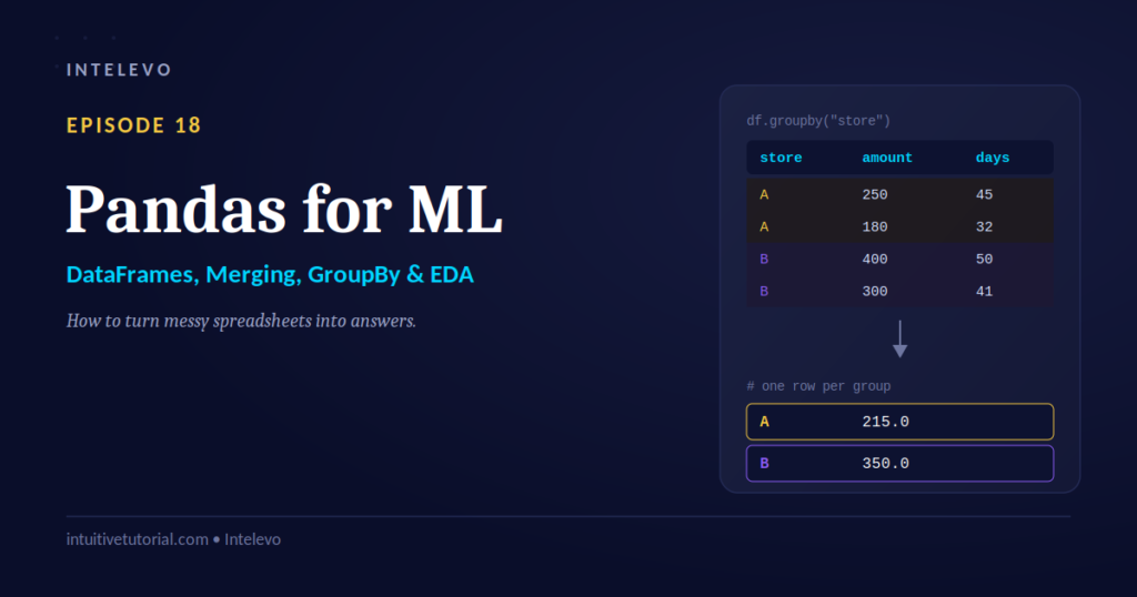
GroupBy works in three steps. First, it splits rows into buckets based on a shared value. Next, it applies the same summary to every bucket. Finally, it combines the results into one small, readable table. Data scientists call this pattern split-apply-combine.
import pandas as pd

sales = pd.DataFrame({
    "store":  ["A", "B", "A", "B"],
    "amount": [250, 400, 180, 300]
})

print(sales.groupby("store")["amount"].mean())
# -> store
#    A    215.0
#    B    350.0
Picture sorting mail by address. Split the letters by destination, apply the same delivery rule to each pile, and combine the results into one organized route. That’s exactly what groupby does with data. Every “average per category” number you’ve ever seen on a dashboard started as a groupby operation just like this one.
One Line, Many Questions
The real power of groupby shows up when you swap the column or the summary function. The same line of code then answers a completely different question.
import pandas as pd

df = pd.DataFrame({
    "class": ["9A", "9B", "9A", "9B"],
    "grade": [88, 92, 79, 85]
})

print(df.groupby("class")["grade"].agg(["mean", "count"]))
#        mean  count
# class
# 9A     83.5      2
# 9B     88.5      2
The agg() function lets you request more than one summary at once. Here, you get the average grade and the headcount, side by side, per group. So, regardless of the category or the summary you need, groupby answers it in a single line.
The Habit That Saves Every ML Project: EDA
Exploratory Data Analysis, or EDA, isn’t a single function. Instead, it’s a habit. Specifically, it’s the quick first look every dataset deserves before it goes anywhere near a model.
import pandas as pd

df = pd.read_csv("students.csv")

df.info()                    # types & missing counts
df.describe()                # min, max, mean per column
df.isnull().sum()            # exactly what's missing
df["class"].value_counts()   # how common is each group
df.info() reveals each column’s data type and how much data is missing. df.describe() shows the minimum, maximum, and mean for every numeric column. df.isnull().sum() tells you exactly what’s missing, column by column. Finally, df["class"].value_counts() shows how common each category actually is.
DataFrames hold the data. Merging brings separate tables together. GroupBy summarizes everything into digestible numbers. EDA, meanwhile, is the habit of checking all of this before you trust any of it. No serious machine learning project skips this step, because it catches real-world surprises before they turn into expensive mistakes.
Common Mistakes Beginners Make
Even with these four building blocks in hand, a few common mistakes trip up new pandas users. Knowing them in advance saves hours of confusing debugging later.
First, beginners often forget to check the how parameter when merging. Without thinking about it, they leave the default inner join in place. As a result, rows silently disappear whenever an ID doesn’t match on both sides. Always ask yourself which rows you want to keep before merging two tables.
Second, many learners skip EDA entirely and jump straight into modeling. This feels faster at first. However, it often means hidden missing values or mismatched types quietly break the model later. A model trained on unchecked data rarely performs well in the real world. Therefore, always run df.info() and df.describe() before doing anything else.
Third, some beginners confuse filtering with looping. They write a manual for loop to check each row one at a time. Pandas, on the other hand, handles this far faster using boolean filtering, like df[df["grade"] >= 85]. Whenever you catch yourself writing a loop over rows, pause and ask whether pandas already has a built-in way to do it.
Finally, new users sometimes forget that groupby returns a special object, not a plain table. You always need to follow it with a summary function, like .mean() or .agg(), before you get a readable result. Once you remember this pattern, split-apply-combine becomes second nature.
Quick Recap: Four Ideas, One Glance
Here’s a fast summary table to anchor everything you just learned.
| Building Block | What It Is | Analogy | In One Line |
|---|---|---|---|
| DataFrames | A labeled table of rows and columns | The class roster | pd.DataFrame({...}) |
| Merging | Combine two tables by a shared ID | Lining up two binders | pd.merge(a, b, on='id') |
| GroupBy | Split, summarize, and combine by category | Sorting mail by address | df.groupby('col').mean() |
| EDA | The first look before modeling | The office clerk’s walk-through | df.describe() |
Test Yourself: Does It Click Yet?
Here’s a quick gut-check question. You have two tables, orders and customers, each containing a customer_id column. What’s the fastest, correct way to combine them into one table?
- A)
pd.merge(orders, customers, on='customer_id') - B)
orders + customers - C) Loop through orders and match manually
- D)
orders.groupby(customers)
The answer is A. pd.merge() lines up both tables on customer_id in a single line. There’s no manual matching and no loop required.
Where You’ve Already Seen This
Interestingly, you’ve used these concepts before, even without realizing it. Consider these everyday examples.
Mail sorting works exactly like grouping. The post office sorts letters by pin code before delivery, which is grouping by a shared value. Spreadsheet VLOOKUP mirrors merging almost exactly, since it pulls a matching row from another sheet using a shared ID. School report cards apply the same split-apply-combine logic as groupby, since they average your marks per subject. Finally, your expense app’s “spent by category” chart is really just a groupby, rendered as a picture.
In other words, DataFrames, merging, groupby, and EDA aren’t locked away inside a coding class. They’re quietly running behind apps you already use every day.
Bringing It All Together
Let’s recap what this episode covered. You learned the four core building blocks: DataFrames, merging, groupby, and EDA. You saw how two separate tables become one, using nothing more than a shared ID. You watched a single line of code summarize thousands of rows by category. Finally, you practiced the first-look habit every real dataset deserves before modeling begins.
Mastering pandas for machine learning doesn’t require memorizing dozens of functions. Instead, it requires understanding these four ideas deeply. Once they click, every messy spreadsheet starts looking like an organized, model-ready table waiting to be built.
What’s Next
In Episode 19, we shift from summarizing data to seeing it. We’ll cover Data Visualization using Matplotlib and Seaborn, turning your rows and summaries into pictures that tell a story at a glance.
If this article helped clarify pandas for machine learning, watch the full video walkthrough on the Intelevo YouTube channel for live code demonstrations. While you’re there, like the video, subscribe to the channel, and drop a comment with your questions. Your feedback genuinely shapes what gets covered next.
See you in the next episode.