Every machine learning model does one thing constantly. It crunches numbers. Lots of them. Millions, sometimes billions, in a single training run. So how does Python handle that kind of scale without slowing to a crawl? The answer is NumPy.
This article is the companion piece to Episode 17 of our Intelevo Machine Learning series, “NumPy for ML.” Watch the full video first for the visual walkthrough, then use this article as your written reference. Take notes, revisit the code, and come back anytime you need a refresher.
By the end of this article, you will understand three core ideas: arrays, vectorized operations, and broadcasting. Together, they explain how NumPy turns Python into a number-crunching machine. Let’s get started.
Why NumPy Matters for Machine Learning
Picture this. You’re decorating five hundred cookies on a tray. You could press a shape into each cookie by hand, one at a time. That works, but it’s slow, and no two presses look exactly alike. Instead, you press one big cutter down on the entire tray. Every cookie gets shaped in a single motion.
That single press, instead of five hundred individual presses, is exactly what NumPy does with numbers. A plain Python list processes numbers one at a time, in a loop. NumPy, however, applies one instruction to an entire array at once. As a result, it runs dramatically faster.
This matters because machine learning models don’t work with single numbers. They work with entire datasets, batches of images, rows of prices, and grids of pixels. Without NumPy, training a model would take hours instead of seconds. With NumPy, Python competes with much faster, lower-level languages for numerical work.
So, before we go further, let’s meet the three ideas that make this possible.
The Three Building Blocks
First, arrays hold the numbers. Think of an array as a container built specifically for numeric data, unlike a general-purpose Python list.
Second, vectorized operations apply one instruction to every number in that array, all at once. No loops required.
Third, broadcasting lets arrays of different shapes work together automatically. A single number can combine with an entire array, and NumPy handles the resizing behind the scenes.
Every time a model processes a batch of data, it leans on these three ideas, repeated millions of times per second. Now, let’s break each one down.
Building Block 1: Arrays
An array is a list of numbers with superpowers. It holds the same shape and the same data type throughout, and it packs everything tightly in memory. That combination makes it fast.
At first glance, an array looks just like a Python list. You still use square brackets. However, the two behave very differently under the hood. A list scatters its items across memory. An array, on the other hand, stores everything in one dense, continuous block. This difference is exactly what gives NumPy its speed advantage.
There’s another key distinction. A Python list can mix data types freely. You can store a number, a string, and a boolean all in the same list. An array cannot. It holds only one data type. That restriction sounds limiting, but it’s actually the trade-off that makes arrays so efficient.
Here’s a quick example:
import numpy as np

prices = [10, 20, 30]      # plain list
arr = np.array(prices)     # NumPy array

print(arr)
print(arr.shape)
# -> [10 20 30]
#    (3,)   <- 3 numbers, one row
Notice the shape attribute. It tells you exactly how the numbers are arranged. In this case, (3,) means three numbers in a single row.
Arrays Aren’t Always Flat
Real machine learning data rarely comes as a single row of numbers. Instead, it often looks like a table of pixels, or even a table of tables. NumPy calls each layer of this structure a dimension. The word “shape” simply counts how many numbers exist along each dimension.
Picture a stack of photographs. One photo is a grid of pixels, which counts as two dimensions: rows and columns. Now stack thirty-two photos together. You’ve added a third dimension, representing how many photos sit in that stack.
import numpy as np

image = np.zeros((28, 28))     # 1 photo
batch = np.zeros((32, 28, 28)) # 32 photos

print(image.shape)
print(batch.shape)
# -> (28, 28)      one grid
#    (32, 28, 28)  32 grids stacked together
Same grid, one more layer on top. That’s the whole idea. If a model can’t hold its data in one organized shape, it simply cannot do math on it efficiently. Arrays solve that problem from the start.
Building Block 2: Vectorized Operations
Now, let’s talk about vectorized operations, the second piece of the puzzle. A vectorized operation applies one instruction to an entire array at once. There’s no loop, no visiting numbers one by one. Instead, the whole tray gets pressed in a single motion, just like our cookie cutter.
Here’s what that looks like in practice:
import numpy as np

scores = np.array([72, 88, 95, 60])
curved = scores + 5

print(curved)
# -> [77 93 100 65]
#    every score bumped, zero loops written
Notice what didn’t happen here. We never wrote a for loop. We simply wrote scores + 5, and NumPy applied that instruction to every score simultaneously. This is the same idea as a loop, conceptually. The difference is timing. Instead of processing numbers one after another, NumPy processes them all together.
Why Loops Slow Down Training
So why should you care about this distinction? Because training a model touches the same numbers millions of times. A Python loop checks each number individually, and that adds up fast. A vectorized operation, meanwhile, hands the entire batch to fast, pre-compiled code running underneath NumPy.
Consider this comparison:
import numpy as np, time

x = np.arange(1_000_000)

start = time.time()
y = x * 2                 # vectorized
print(time.time() - start)
# -> ~0.002 seconds
#    (a loop would take roughly 50x longer)
One million numbers, doubled, in about two milliseconds. A plain Python loop covering the same operation would take roughly fifty times longer. That difference explains why some models train in seconds while others crawl for hours. Vectorization, not raw computing power alone, often makes the difference.
Building Block 3: Broadcasting
Now we reach the third building block: broadcasting. This is where things get genuinely elegant. Broadcasting lets a small array combine with a bigger one. NumPy automatically stretches the smaller array to fit, without copying any data behind the scenes.
Think of it as a cutter that resizes itself. Here’s an example:
import numpy as np

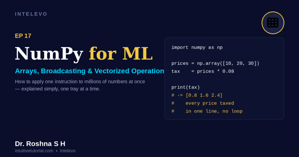
prices = np.array([10, 20, 30])
tax_rate = 0.08              # a single number

tax = prices * tax_rate
print(tax)
# -> [0.8 1.6 2.4]
#    one number "stretched" to match all 3 prices
Notice that tax_rate is just a single number, not an array. Yet NumPy stretches it across all three prices automatically. You never had to write a loop, and you never had to manually resize anything.
The Broadcasting Rule, in Plain English
Broadcasting follows one consistent rule. Line up two shapes from the right. Every dimension must either match exactly, or one of them must equal one. Wherever NumPy sees that one, it stretches the value to fit.
Here’s a more advanced example, closer to real machine learning:
import numpy as np

# 3 photos, each 2x2 pixels
batch = np.ones((3, 2, 2))
bias  = np.array([1, 0])     # shape (2,)

out = batch + bias
print(out.shape)
# -> (3, 2, 2)
#    bias stretched across every photo, every row
This single rule explains how a neural network adds a bias value to every example in a batch, without anyone writing a loop for it. That’s the quiet power of broadcasting. It removes repetitive code while keeping your math correct.
Putting It All Together: A Mini Neural Network Layer
Arrays hold the data. Vectorized operations perform the math. Broadcasting lets differently shaped pieces work together. Chain these three ideas, and you get a working layer of a neural network, in just a few lines of code.
import numpy as np

X = np.array([[1.0, 2.0],
              [3.0, 4.0]])   # 2 samples
W = np.array([0.5, -0.5])    # weights
b = 0.1                      # bias

out = X @ W + b               # vectorized
print(out)
# -> [-0.4  -0.4]
#    both samples processed in one line
That one line, X @ W + b, performs matrix multiplication and adds a bias, and it processes both samples at the same time. This is genuinely how frameworks like PyTorch and TensorFlow operate underneath. They rely on arrays, vectorized math, and broadcasting, just scaled up to millions of numbers across many layers.
The Three Building Blocks, One Glance
Let’s summarize everything in a quick side-by-side view.
| Concept | What It Is | Analogy | In One Line |
|---|---|---|---|
| Arrays | A grid that holds many numbers, one shape | A tray of cookies | np.array([...]) |
| Vectorized Operations | One instruction applied to every number at once | One press of the cutter | arr * 2 |
| Broadcasting | Shapes auto-stretch to fit each other | A cutter that resizes itself | arr + single_number |
Keep this table handy. Whenever you write NumPy code, ask yourself which of these three ideas applies to your problem.
You’ve Seen These Ideas Before
Here’s something worth noticing. These three ideas don’t live only inside a coding class. They quietly power things you use every day.
Consider photo filters on your phone. They apply one filter formula to every pixel at once. That’s a vectorized operation.
Consider spreadsheet autofill. You drag one formula down a column, and it applies to every row. That’s broadcasting a single formula across many cells.
Consider a music equalizer. It boosts every frequency band the same way, in one pass, without manually tweaking each sample.
Even resizing a thousand photos with a single command relies on the same idea. NumPy simply processes the entire grid of pixels as one array, rather than one photo at a time.
A Quick Self-Check
Let’s test your understanding with a quick scenario. Suppose you have prices = np.array([10, 20, 30]), and you want to raise every price by 5. What’s the fastest, correct way to do this in NumPy?
The answer is simple: prices + 5. This single line broadcasts the number 5 across all three prices at once. No loop, and no manual shape matching required. NumPy handles that automatically.
If that answer felt obvious, congratulations. You now understand broadcasting at a practical level.
Common Beginner Mistakes with NumPy
Before we wrap up, let’s cover a few mistakes that trip up most beginners. Knowing them now will save you hours of debugging later.
Mistake one: mixing lists and arrays without converting. A Python list and a NumPy array look similar, but they behave differently. Adding 5 to a list doesn’t work the way you expect. Instead, it either throws an error or concatenates values, depending on the operation. Always convert your data to an array first, using np.array(), before applying math to it.
Mistake two: ignoring shape mismatches. Broadcasting is powerful, but it isn’t magic. Two shapes only combine if they follow the rule we covered earlier: matching dimensions, or a dimension equal to one. If your shapes don’t align, NumPy raises a clear error instead of guessing. Get comfortable printing .shape often. It’s the fastest way to catch bugs before they spread through your code.
Mistake three: writing loops out of habit. Many beginners learn Python through loops, so they naturally reach for a for loop even when NumPy offers a faster, vectorized alternative. Whenever you find yourself looping over an array, pause and ask: can this become one line of vectorized code instead? Usually, the answer is yes.
Mistake four: forgetting data types. Arrays hold one data type throughout. If you mix integers and floating-point numbers, NumPy quietly converts everything to the more flexible type. That’s usually fine, but it can surprise you during precision-sensitive calculations. Check arr.dtype whenever results look slightly off.
Avoid these four mistakes, and you’ll write cleaner, faster NumPy code from day one.
What’s Next: Pandas for Machine Learning
NumPy handles raw numbers beautifully, but real-world data rarely arrives that clean. It shows up in spreadsheets, CSV files, and databases, often messy and full of gaps.
That’s exactly where Episode 18 picks up. We’ll cover Pandas for ML, including DataFrames, merging datasets, groupby operations, and the basics of exploratory data analysis. In short, you’ll learn how to organize, clean, and explore real-world data before it ever reaches a model.
Final Thoughts
NumPy might look intimidating at first, but the core ideas are refreshingly simple. Arrays hold your data. Vectorized operations apply math to everything at once. Broadcasting lets different shapes work together without extra effort.
Once these three ideas click, you’ll read machine learning code with far more confidence. You’ll also write faster, cleaner code yourself, because you’ll instinctively reach for vectorized solutions instead of loops.
If this article helped you, watch the full video walkthrough on the Intelevo YouTube channel for the visual explanation, complete with diagrams and a live code demo. While you’re there, like the video, subscribe to the channel, and share it with someone else learning machine learning. Your questions and feedback are always welcome in the comments section below.
See you in Episode 18, where we explore Pandas for machine learning.
This article is the companion piece to Intelevo Episode 17, “NumPy for ML: Arrays, Broadcasting & Vectorized Operations.” Watch the full video on the Intelevo YouTube channel, and find more tutorials at intuitivetutorial.com.