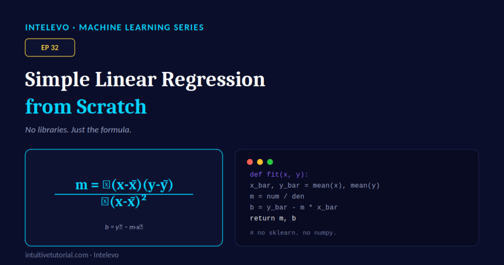
Have you ever called model.fit() and wondered what actually happens inside that single line? This article answers that question completely. By the end, you’ll understand linear regression from scratch, using nothing but averages, one small formula, and plain Python.
This article is the companion piece to Episode 32 of the Intelevo YouTube series. If you’d rather watch it explained visually, check out the video first. Then, return here to review each formula at your own pace.
In the last episode, we met the equation y = mx + b. Scikit-learn found the values of m and b for us instantly. So, today, we remove that convenience entirely. We calculate m and b ourselves, first by hand, then in code.
This exercise matters more than it might first appear. Plenty of data scientists can call fit() and predict() without ever understanding what those functions actually compute. However, once you’ve built the formula yourself, every future regression model you touch becomes transparent, instead of mysterious. You’ll debug faster, tune more confidently, and explain your results more clearly to teammates who ask “but how does it actually work?”
By the time you finish reading, regression will no longer feel like a black box. Instead, it will feel like arithmetic you could do on a napkin.
Quick Recap: Where We Left Off
Let’s refresh three key ideas from the previous episode.
First, regression predicts a number, not a category. Second, our model is simply a straight line, written as y = mx + b. Third, m and b were a mystery last time. Scikit-learn solved for them behind the scenes, without showing us the work.
Today, that mystery ends completely.
Today’s Mission: No Libraries Allowed
Last episode, one line of code did all the heavy lifting:
model.fit(size, price)
That’s convenient, but it hides everything interesting. So, today, we lift the hood. Our mission is simple: calculate m and b ourselves, using nothing but plain Python and basic arithmetic. No imports, no shortcuts. Just the raw formula, step by step.
Two Numbers Decide Everything
Every straight line, regardless of how complex the underlying data looks, boils down to exactly two numbers.
m, the slope, tells us how steeply the line rises. In our house price example, it tells us how much price increases for every extra square foot.
b, the intercept, tells us where the line starts. Specifically, it’s the baseline price before size adds anything at all.
Find m, find b, and you’ve found the entire line. That’s the whole challenge ahead of us.
The Anchor Point: Averages
Here’s a genuinely elegant shortcut. The best-fit line always passes through one very special point: the average of all our x values, paired with the average of all our y values.
Statisticians call these averages x̄ (pronounced “x-bar”) and ȳ (“y-bar”). So, x̄ is simply the average house size in our dataset. Likewise, ȳ is the average price.
Why does this matter so much? Because this anchor point becomes the foundation for both formulas we’re about to build. Once we lock in x̄ and ȳ, calculating the rest becomes remarkably straightforward.
Think of it like balancing a seesaw. If you plotted every single data point and looked for the one point where the data feels perfectly balanced in both directions, you’d land exactly on (x̄, ȳ). Every regression line, no matter how the data is scattered, respects this balance point. That’s not a coincidence — it’s a direct consequence of how the least-squares formula works, and it’s the reason our slope and intercept formulas both lean on these two averages.
The Formula for the Slope
Here’s the one formula that looks the busiest in this entire article:
m = Σ(x − x̄)(y − ȳ) / Σ(x − x̄)²
However, don’t let the symbols intimidate you. Let’s break it into two simple parts.
The top part, or numerator, works like this: for every data point, subtract the average from x, subtract the average from y, then multiply those two differences together. Afterward, add up all those products.
The bottom part, or denominator, works similarly: for every data point, subtract the average from x, then square that difference. Afterward, add up all those squares.
Finally, divide the top by the bottom, and out comes the slope, m.
In plain words, this formula compares how x and y move together, relative to how spread out x is on its own. That’s genuinely all it’s doing.
The Formula for the Intercept
Once you know m, the intercept practically falls into your lap:
b = ȳ − m·x̄
Here’s the intuition behind it. We already know the finished line must pass through our anchor point, (x̄, ȳ). So, we take the average price, then slide back by however much the slope would have added at the average size. Whatever remains is exactly where the line starts. That leftover value is our intercept, b.
Let’s Compute It By Hand
Theory becomes memorable once you work through real numbers. So, let’s use a small, clean dataset: hours studied versus exam score, for five students.
| Hours (x) | Score (y) | x − x̄ | y − ȳ | Product |
|---|---|---|---|---|
| 1 | 30 | -2 | -20 | 40 |
| 2 | 50 | -1 | 0 | 0 |
| 3 | 40 | 0 | -10 | 0 |
| 4 | 60 | 1 | 10 | 10 |
| 5 | 70 | 2 | 20 | 40 |
First, let’s find our averages. x̄ equals 3. ȳ equals 50.
Next, we sum the product column: 40 + 0 + 0 + 10 + 40 = 90.
Then, we square and sum the x-deviation column: 4 + 1 + 0 + 1 + 4 = 10.
So, our slope becomes m = 90 ÷ 10 = 9. Then, our intercept becomes b = 50 − 9×3 = 23.
Just like that, we’ve built a complete regression line entirely by hand: y = 9x + 23.
Plotting Our Hand-Built Line
Numbers on paper are useful, but a chart makes the result feel real. If you plot all five students on a graph, with hours on the bottom axis and score on the side axis, then draw our line through them, you’ll notice something reassuring.
The line doesn’t touch every single point perfectly. That’s completely expected. However, it clearly captures the upward trend in the data. It’s the single best straight line for this exact dataset, and we derived it ourselves, using nothing but arithmetic.
From Formula to Code
Before writing one large block of code, let’s break our formula into three small, honest steps.
First, a mean function adds up a list of numbers and divides by how many there are. Second, a slope function uses those means to calculate m, following our formula exactly. Third, an intercept function uses the slope, along with both means, to calculate b.
Why split things up this way? Because three small functions are far easier to trust and debug than one giant tangle of code. That’s good software practice, not just good math.
Our Regression, Fully From Scratch
Now, let’s see the complete implementation in Python:
def mean(values):
    return sum(values) / len(values)

def fit(x, y):
    x_bar, y_bar = mean(x), mean(y)
    num = sum((xi - x_bar) * (yi - y_bar)
               for xi, yi in zip(x, y))
    den = sum((xi - x_bar) ** 2 for xi in x)
    m = num / den
    b = y_bar - m * x_bar
    return m, b

size  = [850, 1000, 1450, 1800, 2200]
price = [180000, 210000, 268000, 310000, 365000]

m, b = fit(size, price)
print(m, b)   # 133.46  71753.81
Let’s walk through this step by step. First, mean() is exactly one line: sum a list, then divide by its length. We reuse it twice inside fit().
Next, fit() calculates x̄ and y̅ first. After that, it computes the numerator by pairing every x and y together using zip(), subtracting each from its average, multiplying, and summing the results. It computes the denominator the same way, but only for x, squared.
Finally, it divides to get m, then applies our intercept formula to get b. We plug in the exact same house size and price data from Episode 31. Printing m and b gives us roughly 133.46 and 71,753.81.
Notice what’s missing here. No scikit-learn. No numpy. Just loops, sums, and division. And remarkably, it works.
Testing Our Model: Predict and Compare
Let’s put our freshly built model to work.
def predict(x_new, m, b):
    return m * x_new + b

our_price = predict(1600, m, b)
print(our_price)
# 285,283.9
The predict() function is refreshingly simple. It multiplies the new size by m, then adds b. That’s exactly our formula from earlier in this article.
For a 1,600 square foot house, our hand-built formula predicts $285,284. Here’s the genuinely satisfying part: this isn’t a coincidence. Scikit-learn’s LinearRegression uses this exact same ordinary least-squares formula internally. Feed it identical size and price data, and it returns this very same slope, intercept, and prediction. The only difference is that scikit-learn calculates it instantly, instead of showing its work.
Why Build It By Hand First?
At this point, you might wonder why we bothered with all this manual calculation. Here’s why it genuinely matters.
First, there’s no more mystery. Every library call now maps directly to a formula you understand completely. Second, you’ll debug better. When a model misbehaves later, you’ll know exactly what to check, instead of guessing blindly. Third, libraries finally make sense. Scikit-learn isn’t magic. It’s simply this same math, made fast and convenient for everyday use.
There’s also a practical career angle worth mentioning. Interviewers frequently ask candidates to explain how linear regression works, not just how to call it. Having built the formula from scratch yourself, you’ll answer that question with genuine confidence, rather than reciting a memorized definition. That distinction tends to stand out.
Common Pitfalls to Avoid
Before wrapping up, let’s flag a few traps that catch beginners off guard when coding this from scratch.
First, watch out for dividing by zero. If every x value in your dataset is identical, the denominator becomes zero, and your formula breaks. So, always confirm your data actually varies.
Second, avoid mixing up the order of operations. Compute both averages completely before starting the slope calculation. Don’t calculate them partway through a loop.
Third, don’t forget to pair x and y correctly. Each product needs the matching x and y from the same data point. Using zip() keeps everything aligned safely.
Fourth, avoid rounding too early. Round only your final answer for display purposes. Rounding in the middle of a calculation quietly compounds small errors into bigger ones.
Quick Recap
Let’s bring everything together in one glance:
| Concept | In Plain Words |
|---|---|
| Anchor point | The line always passes through the average x and average y |
| Slope formula | m = Σ(x−x̄)(y−ȳ) ÷ Σ(x−x̄)² |
| Intercept formula | b = ȳ − m·x̄ |
| mean(), fit(), predict() | Three small functions, each doing exactly one job |
| No libraries needed | Just loops, sums, and division — the same math scikit-learn runs |
If you remember nothing else from this article, hold onto this table. It captures the entire journey, from raw formula to working code.
Frequently Asked Questions
Why does the slope formula use squared differences in the denominator? Squaring keeps every value positive, so distances from average never cancel each other out. It also happens to produce the exact line that minimizes total squared error, which is precisely what “least squares” regression is named after.
Can this formula handle more than one feature, like size and bedrooms together? Not directly. This particular formula is built specifically for simple linear regression, meaning exactly one input feature. Multiple linear regression uses a related, but more general, approach involving matrix operations. We’ll cover that later in this series.
What happens if my data has no relationship at all between x and y? The numerator in the slope formula ends up close to zero, so m ends up close to zero too. In that case, your “best-fit line” simply flattens out near the average value of y, which honestly reflects that x isn’t a useful predictor.
Do I need NumPy to write this kind of code in practice? No, not for this simple case. Plain Python handles it fine, as this article demonstrates. However, NumPy becomes genuinely valuable once your datasets grow large, since it performs these same sum-based operations far faster under the hood.
Is building from scratch actually necessary before using scikit-learn? Strictly speaking, no. However, doing it at least once, as we did in this episode, pays off enormously in understanding. It turns scikit-learn from a mysterious tool into a fast, convenient shortcut for math you already know.
What’s Next?
Now that you’ve built linear regression from scratch and trust every number it produces, it’s time to bring the shortcut back. In Episode 33, we’ll return to scikit-learn and see exactly how much easier, faster, and more powerful it becomes, once you truly understand what’s happening underneath.
Want to see this exact walkthrough explained visually, with the hand calculation and code demo brought to life on screen? Watch Episode 32 on the Intelevo YouTube channel. Then, subscribe so you don’t miss Episode 33.
Got questions about building regression from scratch? Drop them in the comments on YouTube. We read every single one.