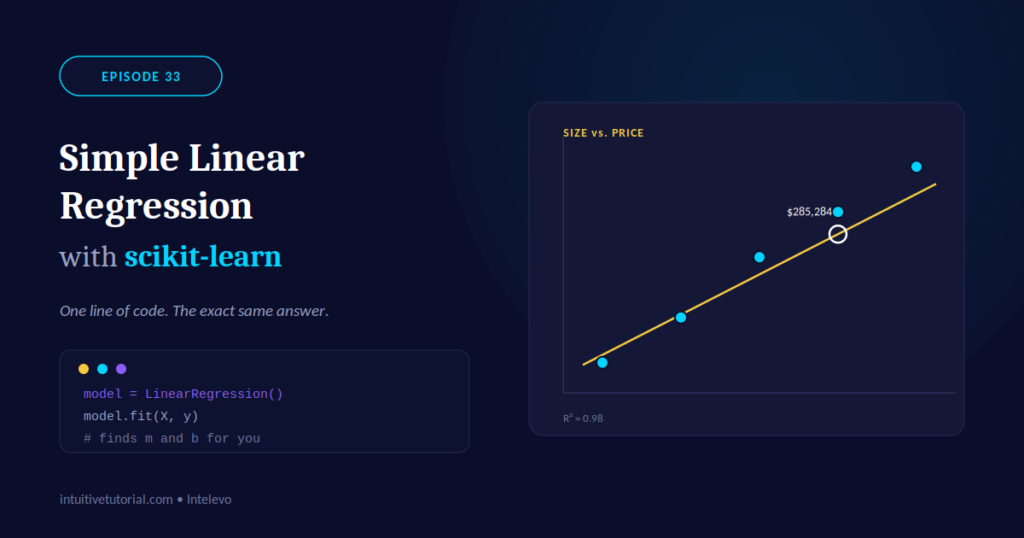
Last time, you built a regression line entirely by hand. You summed numbers, averaged them, and plugged everything into a formula. It worked, but it took effort. Today, you’ll hand that same job to a machine learning library called scikit-learn. It does the work in seconds, and it gets the exact same answer.
This article walks through simple linear regression with scikit-learn, step by step. You’ll see the code, understand what each line does, and watch the model predict a house price you never fed it directly. By the end, you’ll trust the library, because you’ll know it isn’t doing anything mysterious. It’s just doing your math, faster.
A Quick Refresher: What Is Regression, Again?
Before diving into scikit-learn, let’s ground the core idea in one sentence. Regression predicts a number, not a category. It doesn’t sort items into groups, like spam or not spam. Instead, it estimates a continuous value, like a price, a score, or a temperature.
Simple linear regression, specifically, assumes one straight line can describe the relationship between two things. You’ve likely seen its formula before: y equals m x plus b. Here, m represents the slope, and b represents the intercept. Together, these two numbers define exactly where the line sits and how steeply it rises.
Previously, you calculated m and b manually, using sums and averages. That exercise mattered, because it revealed exactly what the model is doing internally. Now, you’ll watch scikit-learn calculate those same two numbers automatically, confirming everything you already learned.
Why Move Beyond Manual Calculations?
Manual regression makes sense for five data points. It teaches you what’s happening under the hood, and that matters. However, real datasets rarely stop at five rows. They stretch into thousands, sometimes millions.
Hand formulas don’t scale well at that size. They’re slow, and small mistakes creep in easily. Also, every real machine learning project needs regression again and again, across different features and different datasets. Retyping formulas each time wastes hours you don’t have.
So, instead of repeating manual math, you reach for a tool built for this exact job. That tool is scikit-learn.
What Is Scikit-learn, Exactly?
Scikit-learn is a free, open-source Python library. Data scientists and engineers use it across the machine learning industry, from startups to large tech companies. Think of it as a toolbox. Rather than forging every tool from raw metal, you simply pick one off the shelf.
This same library powers fraud detection systems, recommendation engines, and forecasting tools worldwide. Importing it takes one line:
from sklearn.linear_model import LinearRegression
That single import gives you access to a fully built, tested, and optimized regression model. Nothing else to write from scratch.
The Dataset: Familiar Faces, New Tool
To keep things consistent, this episode reuses the same five-student dataset from before. Each row represents a house. The first column holds size in square feet, and the second holds sale price in dollars.
sizes  = [1000, 1200, 1400, 1600, 1800]
prices = [200000, 230000, 270000, 300000, 330000]
You already know these numbers. You calculated their slope and intercept by hand previously. That familiarity matters, because it lets you focus entirely on the new tool, not new data.
The Big Picture: Just Three Steps
Before touching any code, here’s the entire workflow in one glance. Scikit-learn regression breaks down into three moves, and nothing more:
- Prepare the data into the shape scikit-learn expects.
- Fit the model so it learns the slope and intercept.
- Predict a value for new, unseen data.
That’s genuinely it. No step gets skipped, and no step is extra. Once you see these three moves clearly, the code stops feeling intimidating.
Step 1: Prepare the Data
Scikit-learn expects your input features, usually called X, in a table format. Even with a single feature, it still wants rows and columns, not a flat list.
Your sizes list, as written above, is flat. So, first, convert it into a NumPy array. Then, reshape it into a column using .reshape(-1, 1).
import numpy as np

X = np.array(sizes).reshape(-1, 1)
y = np.array(prices)

print(X.shape)
# (5, 1)
Here’s why this step matters. One student equals one row. One feature, in this case size, equals one column. Scikit-learn always wants data shaped as rows times columns, even when you only have a single feature to work with. Skip this step, and you’ll hit a shape error immediately.
Step 2: Create and Fit the Model
Next, create an empty model. Then, call .fit() with your prepared X and y.
model = LinearRegression()
model.fit(X, y)
“Fitting” means the model examines every point in your dataset and calculates the slope and intercept that draw the best possible line through them. This is the exact same job you did by hand before. The difference is speed and reliability. One method call replaces an entire page of manual arithmetic.
What Did the Model Actually Learn?
After fitting, you can peek inside the model to see what it found.
print(model.coef_)       # [133.46]
print(model.intercept_)  # 71753.81
Here comes the moment that should build real confidence in this tool. Your hand-calculated values, from manual work earlier, were a slope near 133.46 and an intercept near 71,753.81. Scikit-learn just landed on the exact same numbers.
This proves something important. The library isn’t magic. It runs the same underlying math you already understand, just automated and much faster. Once you see this match, the “black box” feeling around machine learning tools starts to fade.
Step 3: Make a Prediction
Now for the fun part. Ask the model to predict a price for a house size it has never seen directly. Here’s a 1,600 square foot house:
new_house = np.array([[1600]])
predicted = model.predict(new_house)

print(predicted)
# [285284.55]
The model returns $285,284 as its predicted price. Notice something important here: you never typed a formula for this specific calculation. You simply asked, and the model answered, using the pattern it learned during fitting.
How Good Is This Line, Really?
A predicted number alone doesn’t tell you if the model is trustworthy. So, next, check the model’s score using R-squared, often written as R².
print(model.score(X, y))
# 0.98
R² ranges from 0 to 1. A value close to 1 means the line explains the data extremely well. A value close to 0 means the line barely captures any real pattern at all.
In this case, 0.98 means the size of a house explains 98 percent of the variation in its price, according to this dataset. That’s an excellent result for a single-feature model. Naturally, real-world data often looks messier than this, but the interpretation stays the same regardless of the dataset.
The Complete Workflow, In One Glance
Here’s everything together, from import to final score. This is the whole simple linear regression workflow with scikit-learn, condensed into a handful of lines.
import numpy as np
from sklearn.linear_model import LinearRegression

X = np.array(sizes).reshape(-1, 1)
y = np.array(prices)

model = LinearRegression()
model.fit(X, y)

print(model.predict([[1600]]))   # $285,284
print(model.score(X, y))          # 0.98
Read through this block slowly. Notice how each line maps directly back to one of the three big-picture steps: prepare, fit, and predict, with a scoring check added at the end. Nothing here is accidental, and nothing feels overwhelming once you connect each line to its purpose.
Common Mistakes to Avoid
A few traps catch beginners regularly. Knowing them in advance saves real debugging time later.
First, skipping the reshape step causes a shape error. Scikit-learn always expects rows by columns, even for one feature. Forgetting .reshape(-1, 1) triggers an immediate error message.
Second, trusting R² alone can mislead you. A high score on training data doesn’t guarantee good predictions on brand-new data. Always test a model on data it hasn’t seen before, whenever possible.
Third, avoid predicting far outside your original data range. For example, predicting a price for a 10,000 square foot house, when your training data tops out at 1,800 square feet, stretches the line into territory it never actually learned. Extrapolation like this often produces unreliable results.
Fourth, don’t forget to inspect your data before fitting anything. A quick check for missing values, duplicate rows, or obvious outliers saves you from training a model on flawed information. Garbage in still means garbage out, no matter how good the library is.
Where This Exact Pattern Shows Up
This three-step pattern, prepare, fit, predict, repeats constantly across real industries. Consider these examples:
- Real estate: Predicting home prices from size, location, and age.
- HR and salary planning: Estimating fair pay ranges from experience and role.
- Sales forecasting: Projecting expected revenue from advertising spend.
Notice how none of these examples change the underlying workflow. Only the dataset changes. Once you understand simple linear regression with scikit-learn, you already hold the key to dozens of practical, real-world applications.
Quick Knowledge Check
Test your understanding before moving forward. If model.score(X, y) returns 0.35, what does that number actually tell you?
A) The model crashed during training B) The line barely explains the pattern in the data C) The prediction will always be exactly correct D) You need to reshape X again
Take a moment, and think it through before reading further.
The correct answer is B. A score of 0.35 sits much closer to 0 than to 1, which means the line explains only a small portion of the pattern in your data. It’s a working model, technically, but not a strong one.
Recap Table
| Step | Code | Purpose |
|---|---|---|
| Prepare | X = np.array(sizes).reshape(-1, 1) | Shape data into rows and columns |
| Fit | model.fit(X, y) | Learn slope and intercept |
| Predict | model.predict([[1600]]) | Estimate a new value |
| Score | model.score(X, y) | Check how well the line fits |
Keep this table handy. It condenses the entire episode into four rows you can reference anytime.
Frequently Asked Questions
Does scikit-learn calculate the slope differently than manual formulas? No, it doesn’t. Scikit-learn uses ordinary least squares under the hood, the same method you’d use with pen and paper. The library simply automates the arithmetic and handles larger datasets far more efficiently.
Why does X need reshaping, but y doesn’t? Scikit-learn treats X as a table of features, even when you have just one feature. It treats y, the target, as a simple one-dimensional list of answers. That structural difference explains why only X needs reshaping.
Is a high R² score always a good sign? Not necessarily. A high R² on training data can sometimes hide overfitting, especially with more complex models. Always validate performance on separate, unseen data whenever your project allows it.
Can this exact same code handle more than one input feature? Not directly, no. Simple linear regression handles exactly one feature at a time. For multiple features working together, you’ll need multiple linear regression, which the next episode covers in detail.
Do I need to scale or normalize my data before fitting? For simple linear regression with just one feature, scaling usually isn’t necessary. However, once you move to multiple features with very different ranges, scaling often improves both training speed and model stability. Keep that in mind as your projects grow more complex.
What Comes Next: Multiple Linear Regression
One input feature was only the beginning. Real-world prices rarely depend on just size alone. Location matters. Age matters. Number of bedrooms matters too.
In EP34, you’ll explore multiple linear regression. You’ll learn how scikit-learn handles several input features simultaneously, all within that same familiar three-step workflow: prepare, fit, and predict.
Watch the Full Video
Reading builds understanding, but watching builds intuition. The full Intelevo video for this episode walks through every code block on screen, in real time, alongside the reasoning behind each step.
Subscribe to Intelevo on YouTube, and catch the full walkthrough there. If this article helped clarify simple linear regression with scikit-learn, please consider liking the video and leaving a comment. Your feedback genuinely shapes future episodes.
This article accompanies EP33 of the Intelevo machine learning series. Next up: EP34, Multiple Linear Regression.