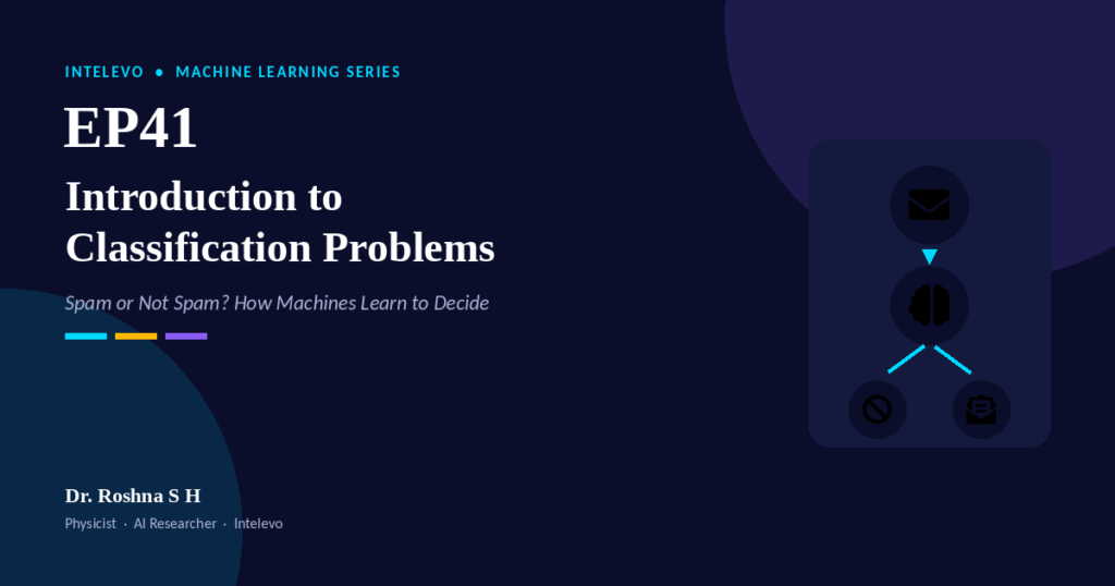
Every email you receive gets a quiet verdict. Your inbox decides: spam, or not spam. You never see that decision happen, but a machine makes it in milliseconds. That single, simple sorting act sits at the heart of classification problems in machine learning — and today, we unpack exactly how it works.
This article accompanies EP41 of the Intelevo Machine Learning series. If you have followed along since EP40, you already know how to predict a number, like a house price. Now, we shift gears completely. Instead of predicting “how much,” we start predicting “which one.” That shift changes everything about how a model thinks, learns, and gets evaluated.
Grab a coffee. Let’s make this genuinely simple.
From Numbers to Categories: A Quick Recap
In EP40, we built a full pipeline to predict house prices. The model took in features like square footage and location, and it returned a number — say, ₹42,50,000. That’s regression. It answers “how much” or “how many.”
Classification asks a completely different question. Instead of a number, it returns a category. Instead of “how much,” it answers “which one.” A spam filter doesn’t tell you how spammy an email is on a scale of one to a hundred. Rather, it makes a call: spam, or not spam.
This distinction matters more than it first appears. Once you separate “how much” from “which one,” entire families of algorithms, metrics, and real-world applications suddenly make sense. Let’s build that intuition step by step.
The One Analogy to Remember: Your Spam Filter
Picture your inbox for a second. New email arrives. Behind the scenes, a classifier looks at the message, weighs the evidence, and sorts it into one of two bins: spam, or not spam.
That’s it. That’s classification in one sentence: given what we observe about something, which group does it belong to?
Throughout this episode, we return to this picture again and again, because it captures every important idea in classification without a single formula. The email is the input. The classifier is the model. Spam and not-spam are the two possible outputs. Simple, right?
Now let’s expand this picture and see how many shapes classification can actually take.
Regression vs. Classification, Side by Side
Before we go deeper, let’s lock in the difference between regression and classification with a direct comparison.
| Regression | Classification | |
|---|---|---|
| Question it answers | “How much?” or “how many?” | “Which one?” or “what type?” |
| Output | A continuous number | A category or class label |
| Example | ₹42,50,000 | “Spam” or “Not Spam” |
| Error measured as | Distance from the true value | Right label vs. wrong label |
Notice how every row flows from one core idea: regression predicts a quantity, while classification predicts an identity. Once that clicks, the rest of this topic becomes far easier to absorb.
Not All Classification Looks the Same
Here’s something many beginners miss: classification isn’t one single shape. It actually comes in three distinct flavors, and each one shows up constantly in real projects.
Binary classification involves exactly two classes. Spam vs. not spam is the classic example. So is approve vs. reject for a loan application.
Multiclass classification, on the other hand, involves one label chosen from several possible classes. Think of a photo classifier deciding between cat, dog, or bird. Only one answer applies, but there are more than two choices.
Multilabel classification allows several labels to apply simultaneously. A movie, for instance, could carry both the “action” tag and the “comedy” tag at the same time. Unlike multiclass, the labels aren’t mutually exclusive here.
Recognizing which flavor you’re dealing with early on saves you from choosing the wrong algorithm or the wrong evaluation metric later.
Classification Is Already Running Your Day
At this point, you might wonder how often classification actually shows up outside a machine learning course. The honest answer: constantly.
Doctors rely on it for medical diagnosis, where a model flags disease as present or absent from scans and vitals. Banks depend on it for credit approval, deciding whether to approve or reject a loan application. Review platforms use it for sentiment analysis, labeling a review as positive, negative, or neutral. Meanwhile, your phone’s camera app uses it constantly for image recognition, telling a cat from a dog from something else entirely.
In other words, classification isn’t a niche academic exercise. It’s already quietly running dozens of decisions in your everyday life.
How Does a Machine Actually Decide?
So how does a model turn raw data into a confident “spam” or “not spam” verdict? The mechanism is more intuitive than most people expect.
A classifier learns from labeled examples where to draw a boundary. Picture a scatter plot: one class of points clusters in one region, and the other class clusters elsewhere. The model’s job is to find a line, or a curve, that separates the two groups as cleanly as possible.
Once that boundary exists, classification becomes remarkably simple. Everything on one side of the line gets one label. Everything on the other side gets the other label. New data doesn’t need a fresh explanation — it just needs a location relative to that boundary.
Three things emerge from this training process. First, the model learns the exact position of the boundary. Second, it learns which side corresponds to which class. Third, and perhaps most interestingly, it learns how confident to be when a point sits close to the middle. You don’t need a heavy formula to grasp this — just the picture. The actual formula behind that boundary is exactly what our next episode, EP42, tackles.
Four Terms Worth Knowing Cold
Before moving further, let’s pin down four words you will hear constantly in classification work.
A feature is a measurable input used to make the decision — word count, sender identity, or number of links inside an email, for instance. A class, sometimes called a label, is the category the model predicts, such as “spam” or “not spam.” The decision boundary is the line or curve the model uses to separate classes. Finally, the threshold is the confidence cut-off used to convert a probability into a final label — usually 50% by default, though not always.
Once these four terms feel natural, reading any classification tutorial or research paper becomes noticeably easier.
Why Not Just Use Regression Here?
A fair question comes up at this stage: why not simply label “not spam” as 0, label “spam” as 1, and fit a straight line through the data? At first glance, it seems like a shortcut.
Unfortunately, this approach runs into two serious problems.
First, the output runs wild. A straight line can easily predict values like -0.4 or 1.8. But “-40% spam” carries no real meaning. We need an answer that stays cleanly between 0% and 100%, and a plain regression line simply doesn’t respect that boundary.
Second, one extreme outlier can tilt everything. A single unusual data point can drag the entire straight line sideways, which shifts the decision boundary for every other point in the dataset too. That’s a fragile, unreliable foundation for a decision that affects real inboxes, real loan applications, or real medical diagnoses.
Because of these issues, classification calls for its own family of algorithms, rather than a repurposed regression line.
A Quick Look at the Toolbox
Thankfully, machine learning already offers a rich toolbox for classification, and this series will explore several of these methods in upcoming episodes.
Logistic regression draws a smooth probability curve between 0 and 1 — and it happens to be exactly what EP42 covers next. Decision trees split data using a sequence of yes-or-no questions, almost like a flowchart. K-nearest neighbors looks at the closest labeled examples in the dataset and lets them vote on the answer. Support vector machines search for the widest possible gap between classes, prioritizing a boundary with maximum breathing room.
Each algorithm approaches the same underlying problem differently, yet all of them ultimately produce that same decision boundary we discussed earlier.
A Callback Worth Remembering: Class Imbalance
Here’s a trap that catches many beginners off guard, and we touched on it earlier in this series: class imbalance.
Imagine 99 out of 100 emails are “not spam.” A lazy model that always guesses “not spam,” without doing any real work, already achieves 99% accuracy. Sounds impressive, right? In reality, that model is completely useless, because it never catches a single spam email.
High accuracy alone, therefore, can quietly hide a broken model. Whenever your dataset skews this heavily, accuracy stops telling the full story. We’ll dig into better metrics for these situations in a later episode, but for now, simply remember to question a suspiciously perfect accuracy score.
Seeing a Classifier in Action: A Python Demo
Theory only goes so far, so let’s translate this into working code using scikit-learn.
from sklearn.datasets import make_classification
from sklearn.model_selection import train_test_split
from sklearn.linear_model import LogisticRegression

# 1. Create a simple two-class dataset
X, y = make_classification(n_samples=200,
                            n_features=2,
                            n_classes=2)

# 2. Split into train and test sets
X_train, X_test, y_train, y_test = \
    train_test_split(X, y, test_size=0.2)

# 3. Train a classifier
model = LogisticRegression()
model.fit(X_train, y_train)

# 4. Predict a label for new data
print(model.predict(X_test[:5]))
# Output: [1 0 0 1 1]   <- class labels
Let’s walk through this step by step. First, make_classification builds a toy dataset containing two features and two classes, which keeps things easy to visualize. Next, train_test_split holds back 20% of the data, so we can test the model fairly on examples it has never seen.
After that, we bring in LogisticRegression from scikit-learn’s linear_model module. Don’t worry about its internal math yet — we’re using it purely as a ready-made classifier here, since EP42 covers that theory in full detail. The line model.fit(X_train, y_train) is where the real learning happens; this single line teaches the model exactly where to place its decision boundary.
Finally, model.predict() takes brand-new, unseen data and returns an array of class labels — ones and zeros in this case. That output is the whole point of classification: not a number, but a clear, confident category.
Three Misconceptions to Drop Right Now
Before wrapping up, let’s clear away three misconceptions that tend to confuse beginners.
First, classification does not only mean two classes. Multiclass and multilabel problems show up just as often as binary ones, so don’t assume every classifier deals with a simple yes-or-no choice.
Second, the model isn’t always fully certain. In fact, most classifiers calculate a probability first, and only then convert that probability into a confident-sounding label. The label you see is simply the model’s best guess based on that underlying probability.
Third, a decision boundary doesn’t have to be a straight line. Depending on the algorithm, it can curve, wiggle, or wrap tightly around clusters of data. The shape of the boundary always depends on which algorithm you choose.
Key Takeaways
Let’s tie everything together before moving on.
Classification predicts a category, not a number, which fundamentally separates it from regression. It comes in three forms — binary, multiclass, and multilabel — and each one appears constantly in real-world systems. Under the hood, a model learns a decision boundary from labeled data, and that boundary is what turns new, unseen data into a confident prediction.
Meanwhile, class imbalance can quietly distort your accuracy numbers, so always question suspiciously high scores. On the practical side, scikit-learn reduces the entire workflow to just a handful of lines of code. And above all, remember that probability comes before the final label — the label is just the confident summary of that probability.
What’s Next: Logistic Regression, Explained
In our next episode, EP42, we finally attach a real formula to today’s spam-filter picture. We’ll meet the sigmoid curve — an S-shaped curve that converts any input into a clean probability between 0 and 1. From there, we’ll see exactly how that probability becomes a final spam or not-spam decision, and I promise to keep the underlying formula as simple as humanly possible.
Frequently Asked Questions
What is the difference between classification and regression? Regression predicts a continuous number, like a price or a temperature. Classification, however, predicts a category or label, like “spam” or “not spam.” The underlying question changes from “how much” to “which one.”
What are the three types of classification problems? The three types are binary (exactly two classes), multiclass (one label from several possible classes), and multilabel (multiple labels can apply at once). Recognizing which type you’re facing shapes your choice of algorithm and metric.
Why can’t you use regular regression for classification? Regression output isn’t bounded, so it can predict impossible values like -40% or 180%. On top of that, a single outlier can tilt the entire boundary. Classification algorithms sidestep both problems by design.
What is a decision boundary in classification? A decision boundary is the line or curve a trained model uses to separate different classes. Everything on one side gets one label; everything on the other side gets the other label.
Is logistic regression used for classification or regression? Despite its name, logistic regression solves classification problems, not regression problems. It calculates a probability, then converts that probability into a class label using a threshold, and we cover this in full in EP42.
Watch the Full Video
This article summarizes the ideas from EP41 of the Intelevo Machine Learning series, hosted by Dr. Roshna S H. For the complete walkthrough, including the visual explanations and live code demo, watch the full video on the Intelevo YouTube channel.
If classification finally clicked for you today, consider liking the video, subscribing to Intelevo, and sharing your questions in the comments. Every comment gets read personally, so don’t hold back.
See you in EP42, where we finally put a formula behind everything we covered here today.