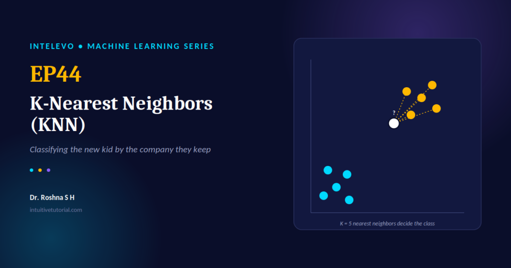
Have you ever judged a stranger by the company they keep? If so, you already understand the core idea behind one of machine learning’s most intuitive tools. The K-Nearest Neighbors algorithm, or KNN, works on exactly that principle. It looks at the data points closest to a new observation, and then it makes a decision based on what those neighbors look like.
This article accompanies EP44 of the Intelevo Machine Learning series on YouTube. If you prefer to watch and listen, the video walks through every diagram and code snippet here. However, this article gives you a text-based reference you can revisit anytime, highlight, or copy code from directly.
By the end of this piece, you will understand exactly how the K-Nearest Neighbors algorithm makes decisions, why the number K matters so much, and how to build one yourself in Python.
The Party Analogy: KNN in One Picture
Imagine you walk into a party where you don’t know a single person. You want to figure out which friend group fits you best. Naturally, you wouldn’t interview every guest in the room. Instead, you’d glance around and notice the five people standing closest to you right now. Then, you’d join whichever group most of those five belong to.
That single instinct is the entire idea behind the K-Nearest Neighbors algorithm. Consequently, once you accept this analogy, the rest of the algorithm becomes almost obvious. KNN doesn’t build a complicated formula. Instead, it simply asks: “Who is closest to this new point, and what are they?”
What Is the K-Nearest Neighbors Algorithm, Really?
At its heart, the K-Nearest Neighbors algorithm is a supervised learning method used for both classification and regression. Unlike Logistic Regression, which we covered in EP42 and EP43, KNN never draws a boundary line through your data. Instead, it stores every training example and waits.
Three ideas define this algorithm completely:
First, KNN has no real training phase. It doesn’t learn coefficients or weights. It just memorizes the dataset and keeps it ready for comparison.
Second, KNN decides by vote. When a new data point arrives, the algorithm looks at its K closest neighbors and copies whatever the majority of them represent.
Third, KNN treats similarity as distance. The algorithm assumes that two points sitting close together on a graph behave similarly. Therefore, distance becomes the single most important calculation in the entire algorithm.
Put simply: tell KNN who your nearest neighbors are, and it will tell you what you are.
How the K-Nearest Neighbors Algorithm Works, Step by Step
The full mechanism breaks down into four clean steps. Once you see them laid out, you’ll notice there is nothing mysterious happening under the hood.
Step 1: Choose a value for K. You decide how many neighbors to consult. A common starting point is five.
Step 2: Measure the distance. The algorithm calculates how far the new point sits from every single point already stored in the training data.
Step 3: Find the closest K neighbors. Next, KNN sorts all those distances and keeps only the smallest K values. These become the “nearest neighbors.”
Step 4: Vote or average. For classification tasks, the majority label among the neighbors wins. For regression tasks, the algorithm averages their numeric values instead.
Notice that no formula ever gets “fitted” to the data in advance. Every new prediction repeats these four steps completely from scratch. As a result, machine learning practitioners often call KNN a “lazy learner,” since it postpones all the real work until prediction time.
A Complete Worked Example
Let’s walk through a full example to see the K-Nearest Neighbors algorithm in action. Picture a simple dataset of fruits, plotted by size on one axis and sweetness on the other. Cyan dots represent apples, and gold dots represent grapes.
Now, a new fruit arrives, and we don’t know what it is. First, we calculate its distance to every point in the dataset. Then, we keep the five closest neighbors, since we chose K equals five for this example.
Among those five nearest neighbors, four turn out to be grapes, and only one turns out to be an apple. Therefore, the majority vote classifies the new fruit as a grape.
Here’s the interesting part. The single closest neighbor to our mystery fruit actually happened to be an apple. However, because we consulted five neighbors instead of just one, the overall verdict remained accurate. This example shows exactly why the “K” in KNN matters so much. It stops a single noisy or unusual data point from misleading your prediction.
Choosing K: The Only Dial You Really Turn
Once you understand the four steps, only one real decision remains: what value should K take? This single choice controls almost everything about how your model behaves.
If K equals one, the algorithm copies the single nearest point exactly. Unfortunately, this makes predictions noisy and jumpy, since outliers can easily throw off the result.
If K equals fifty, on the other hand, the algorithm averages over so many points that it starts ignoring local patterns entirely. Boundaries between classes blur together, and the model becomes too smooth to be useful.
Somewhere in between, say K equals five, you typically find a sweet spot. The model smooths out noise while still respecting the local structure of your data.
A helpful rule of thumb: start near K equals the square root of the number of training points. Additionally, always choose an odd K value for two-class problems. This simple habit prevents ties in the vote and keeps your predictions decisive.
The Math Behind KNN: Euclidean Distance
Every single step of the K-Nearest Neighbors algorithm depends on one question: how far apart are two points? Thankfully, the most common answer uses math you already learned in school.
Euclidean distance calculates the straight-line gap between two points using the Pythagorean theorem:
distance(A, B) = √[ (x₁ − x₂)² + (y₁ − y₂)² ]
This is the same formula you’d use to find the diagonal length between two dots on graph paper. The K-Nearest Neighbors algorithm simply runs this calculation thousands of times, once for every stored point in your dataset.
If your data has more than two features, don’t worry. You just add more squared terms inside the square root, one term for each additional feature. Meanwhile, other distance measures exist too. Manhattan distance and Minkowski distance offer useful alternatives for specific situations, though Euclidean distance remains the default choice for most beginners.
Why Feature Scaling Matters So Much
Here’s a mistake that trips up almost every beginner, so pay close attention to this section. Because KNN measures raw numeric distance, a feature with large numbers can silently overpower a feature with small numbers, even when both features matter equally to the outcome.
Consider comparing income, which might range up to twenty lakh rupees, against age, which only ranges from zero to a hundred. Without scaling, a one lakh rupee gap in income completely overwhelms a forty-year gap in age. Consequently, age becomes almost meaningless to the distance formula, even if age happens to be the better predictor for your problem.
The fix is straightforward. Before running the K-Nearest Neighbors algorithm, rescale every feature to a similar range, typically between zero and one. Tools like StandardScaler or MinMaxScaler from scikit-learn handle this automatically. Make this step a habit every single time you use KNN, without exception.
KNN Isn’t Just for Classification
Many beginners assume the K-Nearest Neighbors algorithm only handles classification problems. However, that assumption sells the algorithm short. KNN also solves regression problems using the exact same four steps we outlined earlier.
The only difference happens at the final step. For classification, say spam detection, the model checks five nearest neighbors: four say spam, one says not spam, so the majority vote predicts spam. For regression, say predicting a house price, the model checks the prices of the five nearest houses: forty two lakh, forty five lakh, forty lakh, forty four lakh, and forty three lakh. Instead of voting, the algorithm averages these numbers, landing on a prediction near forty two point eight lakh.
In other words, the same neighbors, the same distance calculation, and the same core algorithm handle both tasks. Only the final aggregation step changes.
The Lazy Learner Trade-Off: Strengths and Limitations
Because KNN skips training entirely and simply stores raw data, this single design choice creates both its greatest strength and its most significant weakness.
On the positive side, the K-Nearest Neighbors algorithm offers real advantages. It stays simple to understand and explain to non-technical stakeholders. It requires no training time, so you can add fresh data instantly without retraining anything. It naturally handles problems with more than two classes. Finally, it works for both classification and regression tasks without any structural changes.
On the other hand, you should watch out for several limitations. Prediction time slows down considerably on large datasets, since every single prediction requires comparing against the entire stored dataset. The algorithm remains highly sensitive to unscaled features, as we discussed above. It also struggles when your data contains a very large number of features, a problem often called the “curse of dimensionality.” Finally, there’s no universal best value for K. You need to tune it sensibly for each new dataset.
Where You’ll Find KNN in the Real World
The K-Nearest Neighbors algorithm quietly powers many systems you interact with daily. Recommendation engines use it to generate that familiar “customers who bought this also liked” suggestion, essentially finding your nearest taste-neighbors among millions of shoppers.
Fraud detection and credit scoring systems flag suspicious transactions by comparing them against the nearest known fraud patterns in historical data. Image recognition and handwriting recognition systems classify a digit or object by comparing its pixel pattern to thousands of known examples. Additionally, healthcare applications use KNN to support medical diagnosis, matching a patient’s readings against the closest historical cases on record.
Building KNN in Python: A Complete Walkthrough
Now, let’s turn theory into working code. Scikit-learn makes implementing the K-Nearest Neighbors algorithm remarkably simple. Here is a complete example:
from sklearn.neighbors import KNeighborsClassifier
from sklearn.preprocessing import StandardScaler

# 1. Scale features first — distance depends on it
X_train_scaled = StandardScaler().fit_transform(X_train)
X_test_scaled  = StandardScaler().fit(X_train).transform(X_test)

# 2. Choose K and fit — "fitting" just stores the data
model = KNeighborsClassifier(n_neighbors=5)
model.fit(X_train_scaled, y_train)

# 3. Predict by checking the 5 nearest neighbors
predictions = model.predict(X_test_scaled)
Let’s break this down line by line. First, we import KNeighborsClassifier along with StandardScaler, since scaling always comes first when working with distance-based algorithms.
Next, we fit the scaler on our training data and transform it. Then, we apply that same fitted scaler to our test data. This step ensures both datasets sit on identical scales, which keeps our distance calculations fair and accurate.
After that, we choose our value for K and call the fit method. Remember, for KNN, “fitting” doesn’t mean learning a mathematical formula. It simply means storing the training data in memory, ready for comparison later.
Finally, we call predict. Behind the scenes, the model measures distance from each test point to every training point, identifies the five nearest neighbors, and returns a majority vote as the prediction.
That’s the complete model in just a few lines. There’s no gradient descent, no epochs, and no complex optimization loop. The K-Nearest Neighbors algorithm simply remembers everything and compares when asked.
Recap: KNN in One Breath
Let’s tie everything together. The K-Nearest Neighbors algorithm classifies a new point by examining its K closest neighbors and taking a vote. “Close” usually means straight-line, or Euclidean, distance. Always scale your features first, since raw distance calculations get easily fooled by large numbers.
A small K produces a noisy, overfit model, while a large K produces a smooth, underfit one. Therefore, start near K equals the square root of n, and keep K odd whenever possible. Remember, KNN works for regression too, simply by averaging instead of voting. Finally, remember that it behaves as a lazy learner: zero training time, but slower prediction time.
What’s Next in the Series
KNN votes by proximity, and it never draws a boundary line through your data. In our next episode, EP45, we’ll meet a completely different approach to classification: Decision Trees. This model decides through a series of yes-or-no questions, almost like a flowchart built directly from your data. If you found today’s explanation useful, you’ll enjoy seeing how a totally different algorithm can solve the exact same problem.
https://www.youtube.com/@intelevoofficialWatch the Full Video
This article summarizes EP44 of the Intelevo Machine Learning series. For the complete walkthrough, including animated diagrams and a live code demonstration, watch the full video on YouTube. Don’t forget to like the video, subscribe to Intelevo, and share your questions in the comments section below. Your feedback genuinely shapes future episodes in this series.