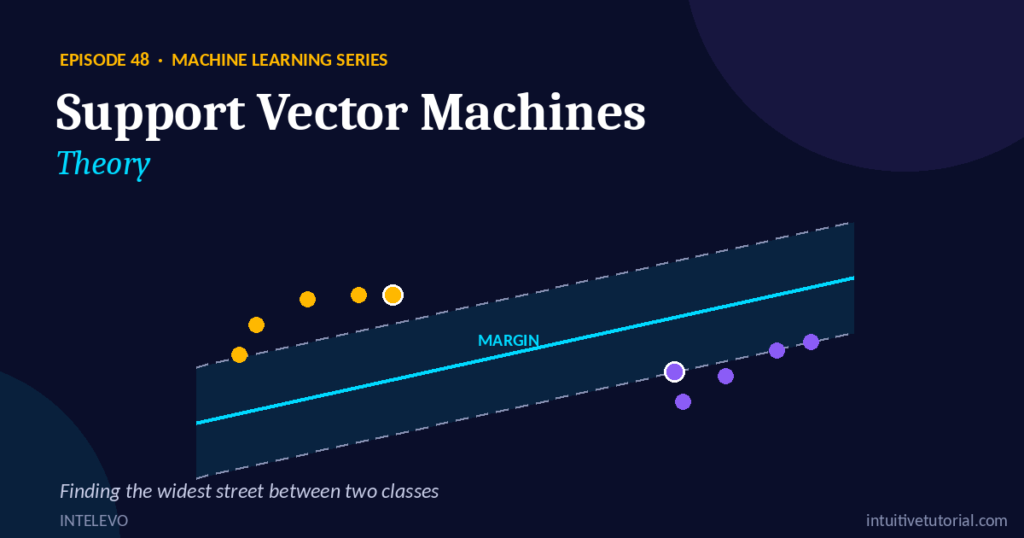
Picture two neighborhoods sitting on opposite sides of a street. Now imagine you need to draw that street as wide as possible, without touching a single house on either side. That single picture captures the entire idea behind Support Vector Machines. This algorithm doesn’t just separate your data; it finds the most confident, most spacious boundary it possibly can.
This article accompanies Episode 48 of the Intelevo Machine Learning series on YouTube. Therefore, if you prefer watching and listening over reading, head to the video first. However, if you like taking notes at your own pace, this article walks through every concept from the episode, in the same order, with the same widest-street analogy.
By the end, Support Vector Machines will feel simple. Let’s get started.
Why Do We Need Support Vector Machines?
Classification problems often look deceptively easy. You have two groups of points, and you need one line to separate them. Consequently, you might think any line that separates them correctly will do the job.
Unfortunately, that assumption breaks down quickly. In most real datasets, dozens of lines can separate two classes correctly. So, which one should you actually pick?
A line that barely squeezes between the two groups works today. But new data rarely looks exactly like your training data. As a result, a fragile boundary risks misclassifying the very next point it sees. This is precisely the gap that Support Vector Machines close.
The Big Idea: Finding the Widest Street
Support Vector Machines don’t settle for just any separating line. Instead, they search for the widest possible corridor between two classes. Then, they draw a single line straight through the center of that corridor.
This corridor has an official name: the margin. We call the center line running through it the hyperplane. In two dimensions, that hyperplane looks like a straight line. In three dimensions, it becomes a flat plane. In higher dimensions, it becomes something we simply call a hyperplane, since human intuition doesn’t easily stretch beyond three axes.
Here’s the key insight: a wider margin means a safer boundary. Consequently, Support Vector Machines actively maximize that width during training, rather than settling for the first valid separator they find.
Three Words That Unlock Everything
Once you understand three terms, the rest of this topic becomes remarkably intuitive.
Hyperplane. This is simply the dividing line itself, sitting at the exact center of the street.
Margin. This is the width of that street, the empty buffer zone with no data points inside it.
Support Vectors. These are the few points that sit right on the edge of the street, touching its curb. They give the algorithm its name for a good reason. Support vectors literally hold the entire boundary in place.
Interestingly, every other point in your dataset could disappear completely, and the boundary would stay exactly where it was. Only the support vectors matter. This single fact explains why Support Vector Machines stay efficient, even on fairly large datasets.
Why a Wider Margin Wins
Let’s compare two scenarios side by side. First, imagine a narrow street that barely fits between two classes. A brand-new point that lands near the middle has a real chance of falling on the wrong side.
Now, picture a wide street instead. The same new point lands safely, comfortably inside its correct zone, with plenty of room to spare.
Consequently, a wider margin gives your model better generalization. In other words, it performs more reliably on data it has never encountered before. That single sentence sums up the entire motivation for maximizing the margin: a wider street is simply a safer, more confident decision boundary.
The One Formula Worth Knowing
Every Support Vector Machine tutorial eventually reaches a formula, so let’s cover it quickly and move on. The objective looks like this:
Minimize ½‖w‖², subject to every point staying on its correct side of the street.
Don’t worry; you will never solve this equation by hand. In plain terms, w represents the tilt and position of your dividing line. A smaller w simply means a wider margin. Meanwhile, scikit-learn’s optimizer handles this calculation instantly behind the scenes.
In plain words, the formula asks one simple question: what is the widest possible street we can draw, while still keeping every point correctly classified? That’s genuinely the whole idea. The rest is implementation detail that your Python library happily takes care of.
Real Data Isn’t Always Tidy
So far, we’ve imagined perfectly separable data. Real datasets, however, rarely cooperate that neatly. A handful of points almost always creep onto the wrong side of the street, no matter how you draw your boundary.
Rather than chasing an impossibly perfect but fragile line, Support Vector Machines allow a small number of these violations. This approach carries a specific name: a soft margin.
A parameter called C controls how much tolerance the model allows. A low C value produces a wider street that tolerates more messiness, resulting in a simpler and safer model. A high C value insists on very few mistakes, producing a narrower, stricter street that can behave more unpredictably if your data contains noise.
Tuning this C parameter properly makes a real difference in practice, and we’ll explore it hands-on in the next episode.
What Happens When a Straight Line Won’t Work?
Sometimes your data refuses to cooperate with any straight boundary at all. Picture one class forming a tight circle, completely surrounded by a ring belonging to the other class. No straight line can separate two groups shaped like that.
This is exactly where the kernel trick becomes useful. Support Vector Machines can lift your data into a higher dimension, similar to lifting a flat photograph into a three-dimensional scene. Once lifted, a flat street can suddenly separate groups that looked impossibly tangled in their original form.
We’ll get fully hands-on with kernels, including linear, polynomial, and RBF options, in the next episode: SVM Implementation and Kernels.
Where You’ll Actually See This Algorithm
Support Vector Machines show up across a surprising range of industries. Spam filters use this technique to separate junk email from genuine messages, based on word patterns. Face detection systems rely on it to decide whether an image patch contains a face or not.
Meanwhile, bioinformatics researchers use Support Vector Machines to classify genes and proteins from raw measurement data. Handwriting recognition systems have also favored this algorithm for years, since it excels at telling similar-looking digits and letters apart.
In short, whenever you need a confident, well-separated boundary between two categories, this algorithm deserves a serious look.
Seeing It Work in Python
Theory becomes much clearer once you see actual code running. Here’s a short script that trains a linear Support Vector Machine using scikit-learn.
from sklearn.svm import SVC
from sklearn.datasets import make_blobs
from sklearn.model_selection import train_test_split

X, y = make_blobs(n_samples=100, centers=2, random_state=42)
X_train, X_test, y_train, y_test = train_test_split(X, y)

# kernel='linear' → a straight street (today's theory)
model = SVC(kernel='linear', C=1.0)
model.fit(X_train, y_train)

print('Accuracy:', model.score(X_test, y_test))
print('Support vectors used:', len(model.support_vectors_))
Let’s walk through this step by step. First, we import SVC, which stands for Support Vector Classifier, along with two helper functions for generating and splitting sample data.
Next, make_blobs generates one hundred points spread across two centers, giving us a clean, simple dataset to experiment with. We then split that data into training and testing sets using train_test_split.
After that, we create our model. Notice the kernel='linear' setting; this keeps our street perfectly straight, matching exactly the theory we’ve covered in this article. The C=1.0 value sets a moderate tolerance for messiness, striking a balance between strict and forgiving.
We call model.fit() to train the classifier on our training data. Finally, we print two results: the accuracy score on our held-out test set, and the number of support vectors the model actually used.
Running this script typically returns an accuracy of 1.0, meaning a perfect score on the test set, alongside a support vector count of around four. Out of seventy-five training points, only four of them actually mattered enough to shape the final boundary. Every other point sat safely on its own side, well clear of the curb.
If you want to explore further, try lowering C to 0.01 and re-running the script. Watch how dramatically the margin widens. You can also print model.coef_ to see the exact numerical tilt of your dividing line, or plot the decision boundary using matplotlib for a visual check.
Strengths and Trade-Offs
Like every algorithm, Support Vector Machines have a sweet spot, along with a few limitations worth knowing upfront.
On the strengths side, this algorithm performs excellently when classes are clearly separable. It also handles datasets with a huge number of features gracefully, which explains its popularity for text classification tasks. Additionally, it stays memory-efficient, since it only needs to store the support vectors rather than the entire training set.
On the trade-offs side, training can slow down considerably on very large datasets. The algorithm also requires properly scaled features to perform well; skipping this step often hurts accuracy significantly. Finally, Support Vector Machines are less interpretable than something like a Decision Tree, where you can literally read off the decision rules one by one.
How SVM Compares to Earlier Episodes
Our classification series has covered several algorithms already, so let’s place Support Vector Machines in context. This comparison genuinely helps you pick the right tool for future projects.
Logistic Regression, covered back in Episode 42, draws a single boundary line too, but it optimizes for probability estimates rather than margin width. Consequently, it doesn’t actively push for the widest possible gap between classes. Support Vector Machines, on the other hand, treat that gap as the entire point of training.
Decision Trees, from Episode 45, take a completely different approach. They split data by asking a sequence of yes-or-no questions, carving the feature space into rectangular regions. This makes trees highly interpretable, since you can literally read off each decision rule. Support Vector Machines sacrifice some of that interpretability in exchange for smoother, more geometric boundaries.
Naive Bayes, from Episode 47, plays the odds using probability and independence assumptions. It trains remarkably fast and handles high-dimensional text data well. However, it doesn’t search for an optimal boundary the way Support Vector Machines do; instead, it simply compares probabilities directly.
So, when should you actually reach for Support Vector Machines? Choose this algorithm when your classes look reasonably separable, and when you want a boundary that generalizes confidently to new data. Avoid it, however, when you need fast training on massive datasets, or when interpretability matters more than raw accuracy.
The Geometry Behind the Curtain
Let’s dig one layer deeper into why maximizing the margin actually works so well. Every point in your dataset sits at some distance from the dividing hyperplane. Mathematically, that distance depends on the vector w and the point’s own coordinates.
Support Vector Machines don’t just care about classifying training points correctly. Instead, they care about classifying them with confidence, meaning a healthy distance from the boundary. As a result, the optimization process naturally pushes the hyperplane as far away from both classes as geometry allows.
This geometric focus explains why Support Vector Machines often outperform simpler linear classifiers on borderline cases. A logistic regression boundary might sit uncomfortably close to a cluster of points, even while classifying every training example correctly. A Support Vector Machine, by contrast, actively avoids that discomfort. It treats proximity to data as a risk worth minimizing, not just an afterthought.
Is SVM still relevant today, given the rise of deep learning? Yes, absolutely. Support Vector Machines remain a strong choice for small to medium datasets, especially when you need a reliable, well-understood algorithm without the overhead of training a neural network.
Do I always need to scale my features before using SVM? In almost every case, yes. Since this algorithm depends heavily on distances between points, unscaled features can distort the margin and hurt your results considerably.
What’s the difference between a hard margin and a soft margin? A hard margin allows zero misclassifications and works only on perfectly separable data. A soft margin, controlled by the C parameter, tolerates a small number of mistakes, making it far more practical for real-world datasets.
Can Support Vector Machines handle more than two classes? Yes, though not directly. Libraries like scikit-learn handle multi-class problems internally, typically using strategies like one-versus-one or one-versus-rest, which combine multiple binary classifiers.
Key Takeaways
Let’s lock in five ideas before wrapping up. First, Support Vector Machines find the widest possible street between two classes. Second, the center of that street is the hyperplane, and its width is the margin. Third, only the closest points, called support vectors, actually decide where the boundary sits. Fourth, soft margins, controlled by the C parameter, let the model tolerate some real-world messiness. Finally, the kernel trick lets this algorithm bend straight streets around curved, tangled data.
Support Vector Machines reward you with a genuinely elegant, geometric way of thinking about classification. Once that widest-street picture clicks, the formulas and code stop feeling intimidating, and start feeling like natural next steps.
Watch the Full Video
This article summarizes Episode 48 of the Intelevo Machine Learning series. For the complete walkthrough, including live diagrams and a full code demonstration, watch the video on YouTube.
If this article helped you, please like the video, subscribe to the channel, and share your thoughts in the comments below. Your feedback genuinely shapes future episodes.
Coming up next, Episode 49 dives into SVM Implementation and Kernels, where we’ll bend the street around curved data and tune the C and gamma parameters hands-on. See you there.