Iterative Policy Evaluation for Estimating Value Function

Introduction

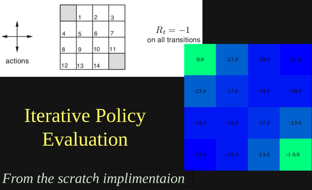
In this tutorial, I am going to code the iterative policy evaluation algotithm from the book “Reinforcement Learning: An Introduction by Andrew Barto and Richard S. Sutton”. I am going to take psuedo code, image and examples from this text. The example I am taking for this tutorial is the gird world maze from Chapter 4 (page 76, example 4.1).

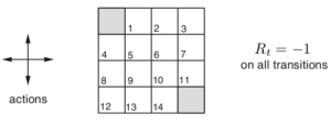
The gird world is a $4$ matrix with the first and last cells are being terminal states. Assuming a random policy, which weights every action equaly, and the only possible actions are up, down, left, or right. For every action except the terminal states the reward will be $-1$. The graphical representation of the rules of the game are shown below.

The psuedo code for the algorithm from the text books is shown below.

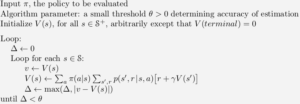
According to this iterative policy evaluation algorithm, if we iterate over the Bellman value function for many times, it will converge to its optimum value. For each states the algorithm looks for the possible actions, next states and rewards and updates the state value at the present state. Since this is an episodic taks (i.e. having terminal states), the discounting is not required. I have written about the intuition (when and why) behind the usage of the discount factor. Please see the post if you are interested in knowing that.

Following is the code for the environment, agent, and algorithm.

Code

import numpy as np
import matplotlib.pyplot as plt

class Env(object):
	def __init__(self):
		self.states = np.zeros((4,4))
		self.fstates = np.zeros((4,4))

	def showEnv(self, aS):
		fig, ax = plt.subplots()
		ax.matshow(self.states, cmap='winter')
		for (i, j), z in np.ndenumerate(self.fstates):
			ax.text(j, i, round(z,5), ha='center', va='center')
		ax.text(aS[1]-0.25, aS[0], ':-)', ha='center', va='center')
		plt.axis('off')
		plt.show()

class Agent(object):
	def __init__(self, start=[0,0]):
		self.start = start
		self.cstate = start
		self.reward = 0.
		self.validActions = ['U','D','L','R']
		self.policy = np.ones((4,4,4))*0.25

	def checkNextState(self, action):
		if action not in self.validActions:
			print('Not a valid action')
		elif action == 'U':
			nstate = [self.cstate[0] - 1, self.cstate[1]]
			self.reward = -1.
		elif action == 'D':
			nstate = [self.cstate[0] + 1, self.cstate[1]]
			self.reward = -1.
		elif action == 'L':
			nstate = [self.cstate[0], self.cstate[1] - 1]
			self.reward = -1.
		elif action == 'R':
			nstate = [self.cstate[0], self.cstate[1] + 1]
			self.reward = -1.
		if (nstate[0] < 0) or (nstate[0] >3) or (nstate[1] < 0) or (nstate[1] >3):
			self.reward = -1.
			nstate = self.cstate
		if nstate == [0, 0]:
			self.reward = 0.
		if nstate == [3, 3]:
			self.reward = 0.
		return nstate

	def takeAction(self, action):
		self.cstate = self.checkNextState(action)
	
	def gpolicy(self, state, a):
		a = ['U','D','L','R'].index(a)
		return self.policy[state[0], state[1], a]

# Iterative Policy Evaluation (Ex. 4.1, p.76 Sutton & Barto)
theta = 2
myEnv = Env()
myAgent = Agent([0,0])
commands = ['U','D','L','R']
delta = 0
k = 0

while True:
	print('Iteration: ', k)
	k+=1
	for (i, j), z in np.ndenumerate(myEnv.states):
		sums = 0
		myAgent.start = [i,j]
		myAgent.cstate = [i,j]
		# print('Agent at ', i, j)
		for act in commands:
			# print('Checking Action: ', act)
			polval = myAgent.gpolicy(myAgent.start, act)
			# print('Policy Prob: ', polval)
			if myAgent.start ==[0,0]:
				step = [0,0]
				myAgent.reward = 0.
				break
			elif myAgent.start == [3,3]:
				step = [3,3]
				myAgent.reward = 0.
				break
			else:
				step = myAgent.checkNextState(act)
			# print('Next Step is: ', step)
			# print('Possible Reward is: ', myAgent.reward)
			sums+=polval * (myAgent.reward+(myEnv.states[step[0],step[1]]))
			# print('Updated Value: ', sums)
		myEnv.fstates[i,j] = sums
		delta = max(delta, abs(z-sums))
		# print(delta)
		# myEnv.showEnv(myAgent.cstate)
	myEnv.states = myEnv.fstates
	print(myEnv.fstates)
	if delta>theta:
		break
	if k > 1000:
		break

After each iteration, the value function is printed. We can see it converges towards the following value.

Iteration:  1000
[[  0. -13. -19. -21.]
 [-13. -17. -19. -19.]
 [-19. -19. -17. -13.]
 [-21. -19. -13.   0.]]

A visual representation of the same might make more sense.

myEnv.showEnv(myAgent.cstate)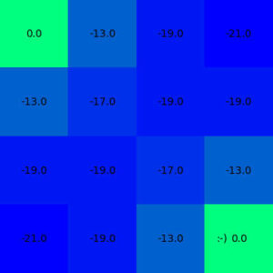

Conclusion

As we can see here the converged value function after iterative policy evaluation is symmetric and resonates the reward rule. States next to terminal states are having same values. The agent will be learning to reach a terminal as soon as possible. Hence the value function around the center of the gird are low and relatively high near the terminal states.

The converged values are just one value different than the result shown in the text book. I think this is because we are following an iterative approximation method rather than solving linear equations directly. We can see that our solution gets very close to the analytical one shown in the text book.