This article shows two key visual intuitions behind the usage of a discount factor in reinforcement learning with image, code, and video.
Introduction
Most of the advances in science and technology happened in the last 100 years. We can see mind-boggling progress in automotive, medicine, communication, energy, etc. . Among these advances, some technologies shake and reform every other. For example, computers penetrated every other field, catalyzed, and reshaped the way they are now.
I often think it is the generic nature of those inventions that make them so lethal. After computers and the internet, the potential revolution is going to be Artificial General Intelligence (AGI).
Algorithms that are capable of doing specialized tasks are already part of our life. For example, recommendation systems help us in retail, finance, media, etc.. We have algorithms good with language translation, speech recognition, automated driving, etc. In general, Machine Learning (ML) algorithms leverage patterns in data to make reliable predictions and create value. All of this happened because we accumulated a massive amount of data that resulted from the computing revolution.
We can see two main philosophies that are fundamental to these learning algorithms. One is learning from diverse examples (supervised learning) and the other is learning from trial and error (reinforcement learning).
Reinforcement Learning
In Reinforcement Learning (RL), the agent learns from trial and error. RL theory formulates the problem such that the agent gets incentives to achieve a goal.
The agent moves from state to state by observing the environment, taking actions, and receiving rewards at every step. Desirable actions result in high rewards while undesirable actions result in low ones.
The rewards could be represented as $R_t, R_{t+1}, R_{t+2},…+R_{t+n-1}$ at every $t$ step, where the agent may achieve its final goal in the $n$th step. Such a session is often called an episode.
Please note that it is also possible for the session to continue infinitely (i.e., $n\to\infty$). The task for the agent is to collect as many high rewards as possible. Mathematically it is represented as the sum of all rewards $R_{t}+R_{t+1}+R_{t+2}+…+R_{t+n-1}$.
You might recognize this as in the form of a mathematical series (addition of a series of infinite numbers). Mathematical analysis is a branch of mathematics (like trigonometry, calculus, linear algebra) that studies such objects.
Discount factor
However, in the infinite session case, an additional challenge is that the sum of rewards keeps growing. This problem is known as unboundedness in mathematical terms. We can’t deal with such unbounded functions/signals computationally. And we need a solution for this.
The discount factor (a number between 0-1) is a clever way to scale down the rewards more and more after each step so that, the total sum remains bounded. The discounted sum of rewards is called return ($G_t$) in RL.
$G_t = R_t+\gamma R_{t+1}+\gamma^2R_{t+2}+\gamma^3R_{t+3}+…$
Let us see a visual intuition on why this works. For example, the series $\frac{1}{2}+\frac{1}{4}+\frac{1}{8}+…$ is a geometric series. The following figure represents it visually.
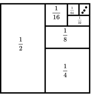
Here each term or rectangle here is half of its preceding one. As you can see the limit of such an infinite sum of such terms will be 1 in this example. In this specific example, the ratio between successive terms was $\frac{1}{2}$. And we were lucky to represent such a pattern in visual form.
Likewise, the series of gammas forms a geometric series. Here the ratio between two consecutive terms is $\gamma$ itself. The sum of such gamma series generalizes to a solution as shown below.
$1+\gamma+\gamma^2+\gamma^3+…=\frac{1}{1-\gamma}$ as long as $\lvert \gamma \rvert<1$.
This makes sure that even if the reward remained high and consistent (for example $R$) at every step, the cumulative discounted sum of it will be bounded.
$R+\gamma R+\gamma^2R+\gamma^3R+…= \frac{R}{1-\gamma}$
Other than making the return bounded, it got one additional advantage as well. It can adjust the behavior of the agent to focus on long-term goals or short term. For example, if we assume that $\gamma$ was 0, we can see that all terms in the above equation, except the first one, go to zero. This means now the focus of the agent will be on the immediate reward only and not on long term rewards.
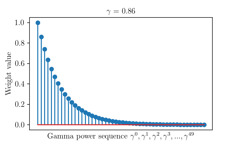
The following code snippet generates pictures that show how the discount factor terms ($\gamma^0, \gamma^1, \gamma^2, \gamma^3, .., \gamma^{49}$) change for different values of $\gamma$ from 0 to 1.
import numpy as np
import matplotlib.pyplot as plt

labelsize = 12

width = 5
height = width / 1.618

plt.rc('font', family='serif')
plt.rc('text', usetex=True)
plt.rc('xtick', labelsize=labelsize)
plt.rc('ytick', labelsize=labelsize)
plt.rc('axes', labelsize=labelsize)

gammas = np.arange(0,1,1.0/100)

i = 1
def animator(gamma, i):
	fig1, ax = plt.subplots()
	weight_terms = [np.power(gamma, k) for k in range(0,50)]
	plt.stem(weight_terms, use_line_collection= True)
	plt.xticks([])
	plt.title('$\gamma$ = {}'.format(round(gamma,2)))
	plt.ylabel('Weight value')
	plt.xlabel('Gamma power sequence '+ '$\gamma^0, \gamma^1, \gamma^2,\gamma^3, ...,\gamma^{49}$')
	fig1.set_size_inches(width, height)
	plt.savefig('dynamicGammaSequence'+str("{0:0=4d}".format(i))+'.png', dpi = 200)
	plt.close()

for gamma in gammas:
	animator(gamma, i)
	print('Saving frame: ', i)
	i+=1
The change of weights is shown in the video below.
If you found this article helpful and would like to help me financially so that I can write more such content, you can do it via paypal.me/cksajil