Introduction
In this post, let’s take a look at the intuition behind Naive Bayes Classifier used in machine learning. Naive Bayes classifier is one of the basic algorithms often encountered in machine learning applications.
If linear regression was based on concepts from linear algebra and calculus, naive Bayes classifier mostly backed up by probability theory. This topic nicely captures a few of the fundamental probability and associated concepts which occur frequently in machine learning.
Let’s start with the popular classification task naive Bayes accomplishes.
Classification is one of the tasks which humans were able to teach machines. All of our emails classify every incoming email as spam or not every time a new email comes. Financial institutions like Banks monitor all their transactions algorithmically to detect any fraudulent behavior.
Naive Bayes is one such algorithm that is often employed to accomplish such tasks.
Before getting into the nuts and bolts of it, let’s take a look at its history.
History
The cornerstone of the naive Bayes classifier is the Bayes rule which was invented by Thomas Bayes. He was an English statistician and philosopher who proposed the mathematical relation also called inverse probability.
It has a different perspective on the probability of events compared to a frequentist point of view.
Rather than thinking of probability values as a fixed ones, the approach is to update our belief after we encounter data/observation. Let’s see how the naive Bayes classifier makes use of this approach.
Key Intuition
The only key intuition/crux idea here is “Inference in light of evidence”
Let me elaborate on what do I mean by this. Suppose you are in a restaurant ordering food. If you are new to the restaurant, your choice for a meal might be a random pick. But if you are a regular visitor there you might order something different than what you ate last day. The item you ate yesterday had a role in your choice of today’s meal.
Dependent Events and Conditional Probability
In simple terms, this represents the dependence of events. When two events are independent, the probability of occurring one does not affect the other. This leads us to the cornerstone concept behind the naive Bayes classifier called Conditional Probability.
Suppose you have two fair coins. If you toss both, the probability of getting head for the second coin is 0.5 regardless of the outcome of the first coin. This is because the first event in no way affects or influence the second.
Now consider the example of a dice. The chance of getting the number 2 is $\frac{1}{6}$ as you know. Let’s look at what is happening here visually.

The figure gives a visual representation of discrete probability as the ratio between areas of the event under consideration and total sample space.
If I give you the additional information that the number got was even, what is the probability of getting 2 now?. Let us look at what is happening visually.
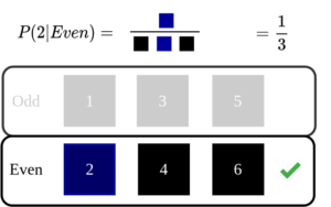
Here the additional information helps us to narrow down our sample space by half.
We can think of it this way. Dependent events–> gives additional information–> helps us to narrow down sample space.
What if the additional information was “the number is an integer”. Does it say any additional information that will helps us narrow down the sample space?.
$$P(2|\text{it is an integer})=\frac{1}{6}$$
Here it does not give any additional information. Even if we go with the traditional equation $$P(A|B)=\frac{P(A \cap B)}{P(B)}$$
$$P(2|\text{it is an integer})=\frac{P(2 \cap \text{it is an integer})}{P(\text{it is an integer})}$$
$$= \frac{\frac{1}{6} \cdot 1}{1}= \frac{1}{6}$$
Because we always get an integer when we roll a dice.
Hence, Independent events–> do not give additional information–> do not help us to narrow down sample space.
Such examples of conditional probability are easy since we could directly narrow down our sample space. But not all situations are like this. Let us consider one such example.
The Bayes Theorem
Let us consider one of the popular examples of Bayes theorem. Consider there are 200 farmers and 10 librarians in a village. For simplicity, we can assume that there are only farmers and librarians in the village.
Suppose 40 % of librarians are tidy which means 60% of them are not tidy. When it comes to farmers the pattern is different. 10% of farmers are tidy while 90% of them are not. Let’s have a visual representation of the scenario.

According to our data
$P(\text{Librarian}) = \frac{10}{210} = \frac{1}{21} = 4.76\%$
and $P(\text{Farmer}) = \frac{200}{210} = \frac{20}{21} = 95.23\%$
Now let’s look at one conditional probability situation here. What is the probability of a person to be a librarian given he or she is tidy? i.e. $P(\text{Librarian|Tidy})$
Here the information regarding tidy/not tidy definitely gives additional information but the difference is the tidy behavior depends on whether it is farmers group or librarians group.
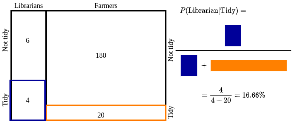
In traditonal equation form we can represent this as:
$P(L|T) = \frac{P(T|L) \cdot P(L)}{P(T)}$
Here the numerator is the Blue part and denominator is the sum of Blue and Orange areas.
Please note that how it updated our belief about a random person chosen among the group to be a librarian. Initially, it was 4.76%. Now the additional information that the person is tidy increased it to 16.66%. This connects back to our key intuition. We made inference in light of the evidence.
What if the information given was the person was not tidy. Then $P(\text{Librarian|not Tidy})$ will be $\frac{6}{6+180} = 3.23\%$.
Note how the Bayesian philosophy takes a flexible approach towards probability estimate while Frequentist remains rather conservative. The initial belief is called the prior probability and the updated inference is called the posterior probability. The $P(T|L)$ part is known as the likelihood.
Difference Between Conditional Probability and Bayes Theorem
We can see that in the conditional probability example, the denominator area calculation is obvious and easy. But in the Bayes example, it includes a bit more careful calculation.
Essentially conditional probability and Bayes theorem are the same. The only technical difference is in the denominator part. If the denominator can be directly computable then we call it simply conditional probability.
In more formal mathematical terms we can say that conditional probability is a generalization of the Bayes rule.
Bayes Classifier From Scratch
Let us consider how we can apply these concepts to do classification with real datasets. When it comes to real data sets, the problem formulation will be like shown below.
$P(\text{Class|Data}) = \frac{P(\text{Data|Class})P(\text{Class})}{P(\text{Data})}$
Here given a new datapoint, we want to predict which class it belongs to. In the earlier Bayes example where we had only two variables involved (Job & Cleanliness). But real-life datasets will have multiple features for each data point. This updates the formula as
$P(C|d_1, d_2,…, d_n) = \frac{P(d_1, d_2,…,d_n|C)P(C)}{P(D)}$
Since the independence assumption of features, we can expand the numerator part.
$P(C|d_1, d_2,…, d_n) = \frac{P(d_1|C) \cdot P(d_2|C) … P(d_n|C) P(C)}{P(D)}$
For each class in the dataset, we can calculate this posterior probability value. The class with maximum value will be our prediction. This is represented mathematically as shown below.
$C = argmax_CP(C|D) = P(d_1|C) \cdot P(d_2|C) … P(d_n|C) P(C) $
Please note that the denominator is ignored because it is constant.
Since all of these are probability values (0-1) and we are multiplying them, taking the log of the value will make the computation easy. The few advantages of taking log include the ability to handle small fractions, prevent underflow, multiplication to be turned to addition, emphasise large and small values in a non-linear fashion.
This updates the equation as shown below.
$C = argmax_C log(P(d_1|C))+ log(P(d_2|C))+ …$
$+log( P(d_n|C))+log( P(C)) $
To compute the likelihood for each datapoint. We can model it assuming each feature is normally distributed with mean and standard deviation values. Depending on the class we can compute it from our model.
As a sanity check, the following figures show the histograms of both features fitted with Gaussian curves.


The equation for Gaussian distribution with a given mean and standard deviation is shown below.
$P(d; \mu, \sigma) = \frac{1}{\sigma \sqrt{2 \cdot \pi}}e^{-\frac{(d – \mu)^2}{2 \sigma^2}}$
Depending on the data, class, and feature we can compute the respective likelihood value, then take logarithm. The class which gives the maximum sum of likelihood will be predicted as output.
For the implementation, we can consider the simple Iris dataset.
This dataset contains dimensions of three types of flowers. Hence the label will be one of the three classes. For simplicity, let’s take only the first two features. Before moving further let’s inspect how is the distribution of labels in our dataset.
# import Libraries
from sklearn import datasets
import numpy as np
import matplotlib.pyplot as plt
from sklearn.model_selection import train_test_split
from collections import Counter
import pandas as pd


# Load Iris dataset
iris = datasets.load_iris()

# For Simplicity let's consider only two features
X = iris.data[:, :2]
y = iris.target

N = X.shape[0]

# Do the Train and Validation Test Split
X_train, X_test, y_train, y_test = train_test_split(X, y, test_size=0.2)

#Count the #of occurance of each flowers
c = Counter(y)
labels = np.array(list(c.keys()))
freq = np.array(list(c.values()))/N

#Plot the frequency histogram
fig1, ax = plt.subplots()
fig1.subplots_adjust(left=.16, bottom=.2, right=.99, top=.97)

plt.bar(labels, freq)
plt.xticks([0,1,2])
plt.xlabel('Flower Types')
plt.ylabel('% of occurance')
fig1.set_size_inches(4, 2.5)
plt.savefig('IrisClassDistribution.png', dpi = 100)
plt.close()

As we can see here our dataset is balanced and each flower appears around the same frequency.
This means even if we predicted randomly between the three classes, we are expected to get an accuracy of around 33% as a baseline. The following code verifies that empirically.
from sklearn.metrics import accuracy_score

def blindPrediction(data):
	m = data.shape[0]
	predictions = []
	for i in range(m):
		predictions.append(np.random.choice([0,1,2]))
	return predictions

acc = []
K = 1000
for i in range(K):
	blindpred = blindPrediction(X_test)
	acc.append(accuracy_score(y_test, blindpred))

fig2, ax 	= plt.subplots()
fig2.subplots_adjust(left=.16, bottom=.2, right=.99, top=.97)
plt.hist(acc, bins =20)
plt.xlabel('Accuracy')
plt.ylabel('Count')
fig2.set_size_inches(4, 2.5)
plt.savefig('empiricalAccuracy.png', dpi = 100)
plt.close()

As you can see here we just followed our blind prediction strategy and most of the time we were able to get an accuracy of at least 33%.
This means our new classifier should atleast perform better than this baseline. Now let’s get back to the implementation of our classifier.
Code
Since all classes are balanced we can assume our prior probability as 0.33.
In our homemade classifier, we will capture all calculations under a custom naive Bayes classifier class. The following code accepts the training data, computes Gaussian mean and standard deviation under each class, and finds the class which maximizes the likelihood of observing the given test data
# import Libraries
import numpy as np
from sklearn import datasets
from collections import Counter
from sklearn.metrics import accuracy_score
from sklearn.model_selection import train_test_split


# Load Iris dataset
iris = datasets.load_iris()


# For Simplicity let's consider only two features
X = iris.data[:, :2]
y = iris.target


# Do the Train and Validation Test Split
X_train, X_test, y_train, y_test = train_test_split(X, y, test_size=0.2)


# Define out custon Naive Bayes Classifier
class myNBClassifier(object):
	"""Custom Naive Bayes Classifier"""
	def __init__(self):
		self.means = []
		self.stds =  []


	def myGaussian(self, x, mu, sig):
		"""Gaussian function to compute likelihood"""
		lhd = 1/(sig * np.sqrt(2 * np.pi))*np.exp(- (x - mu )**2 / (2 * sig**2) )
		return lhd

	def fit(self, data, label):
		"""Train our model with training data and labels given"""
		self.c = list(Counter(y).keys())
		dataset = np.column_stack((data, label))

		for g in self.c:
			segment = dataset[dataset[:,2]==g][:,:-1]
			f1, f2 = np.hsplit(segment,2)
			self.means.append([np.round(np.mean(f1),2),np.round(np.mean(f2),2)])
			self.stds.append([np.round(np.std(f1),2),np.round(np.std(f2),2)])


	def predict(self, data):
		"""Predict the class for a given set of inputs"""
		fn =data.shape[1]
		mypred = []
		for row in data:
			likelihood = []
			for l in self.c:
				mus = self.means[l]
				sigs = self.stds[l]
				lkd = 0
				for i in range(fn):
					lkd+=np.log(self.myGaussian(row[i], mus[i], sigs[i]))
				likelihood.append(lkd+np.log(1./len(self.c)))
			mypred.append(np.argmax(likelihood))

		return np.asarray(mypred)


# Create an instance of our Classifier
myNB = myNBClassifier()

# Train with training data
myNB.fit(X_train, y_train)

# Predict class for test data
pred = myNB.predict(X_test)

# Compute the accuracy
acc = accuracy_score(y_test, pred)*100

# Print out the accuracy of our classifier
print("Accuracy of our model: {}%".format(np.round(acc, 2)))
Output
Accuracy of our model: 80.0%
As you can see, we get an accuracy of around 80%. Please note that our model is designed to work with only two features. Not all best coding practices are followed here but our focus was to understand the internals working of the Naive Bayes classifier.
Conclusion
We started from the fundamental probability concepts, Bayes theorem, and extended it to real-life datasets. We built from the scratch implementation of our Naive Bayes classifier on top of these concepts.
We can still explore questions like what will happen to our classifier performance if we relax the independence assumption and assumption about Gaussian distribution of features etc. That is for another day.
Thank you for your time.