In one of our earlier posts, we have seen how we can visually relate the parts of the one-dimensional Gaussian distribution equation.
In this post, we will follow the same strategy to understand the terms that comes up with a Multivariable Gaussian distribution. We will focus on the Bivariate Gaussian distribution as distributions of higher-order becomes almost impossible to visualize.
Let us have a quick look at the general form of Multivariate Gaussian distribution equation.
$f(x) = \frac{1}{\sqrt{(2\pi)^n|\boldsymbol\Sigma|}}
\exp\left(-\frac{1}{2}({x}-{\mu})^T{\boldsymbol\Sigma}^{-1}({x}-{\mu})
\right)$
If we compare it with the univariate case which is,
$f(x)=\frac{1}{\sqrt{2\pi}\sigma}
\exp\left(-\frac{1}{2}\frac{({x}-{\mu})^2}{\sigma^2}\right),$
For the single variable case, it was a bell-shaped curve. But in the bivariate case, we can think of it as a three-dimensional surface curve peaking at its mean center.
For the same reason, the $\boldsymbol x$ data points will be a tuple of values $(x_1, x_2)$, denoting their location. Depending on the point’s proximity to the mean center the amplitude of the same starts to peak.
Compared to the single variable case, how far is a point is from the mean center depends on the direction also. Since $\boldsymbol x$ has two components $x_1$ and $x_2$ the sense of direction comes up here. We have written about the vectors and abstract direction in one of our earlier posts.
Varaiance to Covariance Matrix
In the univariate case, we had the variance ($\sigma^2$) to denote the spread of the data. Higher $\sigma^2$ means high variance and spread of data.
The bivariate equivalent of $\sigma^2$ here is the $2\times2$ covariance matrix.
A Bit of Linear Algebra
To understand how the covariance matrix deals with different points depending upon their position is based on linear algebra. It is important to understand matrices as linear transformations applied to vectors in a plane. For example, a unit matrix is identical to the multiplicative identity equivalent of one in a number system.
This means if we multiply any vector with a unit matrix, we will get the vector itself as output.
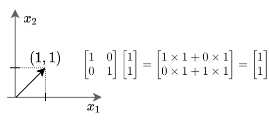
Here we can see the vector $x$ stays unchanged after being multiplied by the unit matrix.
In multivariate Gaussian distributions, it is the covariance matrix that holds the key to the spread of data and the direction of spread. The technical definition of covariance tells us that it contains the covariance between each pair of elements of a given random vector. Hence it will be a square matrix and every diagonal element will be the variance of the random vector itself.
The covariance equation can be written as:
$\sigma(x, y) = \frac{1}{n-1} \sum^{n}_{i=1}{(x_i-\bar{x})(y_i-\bar{y})}$
One additional point to be noted is the symmetric property of the covariance matrix. This is because $\sigma(x_i, x_j) = \sigma(x_j, x_i)
$.
Written in matrix form the covariance matrix is:
$\Sigma = \left( \begin{array}{ccc} \sigma(x_i, x_i) & \sigma(x_i, x_j) \\ \sigma(x_j ,x_i) & \sigma(x_j, x_j) \end{array} \right)$
Now let’s take a look at how the covariance matrix of two vectors that are not correlated will look like.
The following code generates two random vectors of 500 elements each, normally distributed with zero mean and unit variance. The code plots the scatter plot of both the vectors and prints the covariance matrix.
import numpy as np
import matplotlib.pyplot as plt

# Set values for clean data visualization
labelsize 	= 12
width 		= 4
height 		= 4

plt.rc('font', family ='serif')
plt.rc('text', usetex = True)
plt.rc('xtick', labelsize = labelsize)
plt.rc('ytick', labelsize = labelsize)
plt.rc('axes', labelsize = labelsize)

fig1, ax 	= plt.subplots()
fig1.subplots_adjust(left=.16, bottom=.2, right=.99, top=.97)

# Normal distributed x and y vector with mean 0 and standard deviation 1
x1 = np.random.normal(0, 1, 500)
x2 = np.random.normal(0, 1, 500)
X = np.stack((x1, x2), axis=0)


plt.scatter(x1, x2, color = 'k')
plt.xlabel('$x_1$')
plt.ylabel('$x_2$')

fig1.set_size_inches(width, height)
plt.savefig('RandomScatter.jpeg', dpi = 300)
plt.close()

print(np.cov(X))
Lets look at the scatter plot first.
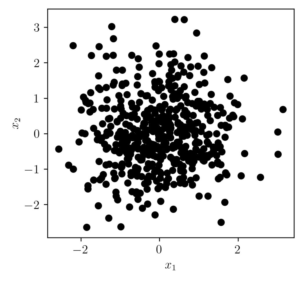
As we can see from the graph, we don’t see any correlation/trend between the two vectors. Also, the covariance matrix output is shown below.
[[0.94868231 0.03279231]
 [0.03279231 1.05590377]]
We can see here the $\sigma(x, x)$ and $\sigma(y,y)$ as nearly equals one and the $\sigma(x,y)$ and $\sigma(y,x)$ as same and nearly equals zero also.
The Crux Idea
In our earlier post about single variable Gaussian distribution, we have shown how the negative exponent ($e^{-x}$) is boosting up or attenuating down depending upon the value of $x$. The key difference in the bivariate case is that the covariance matrix plays a role in determining which data point from the vector $(x_i, x_j)$ should be boosted up or attenuated.
Now let us look at the code to generate a bivariate Gaussian distribution with a given mean and covariance matrix values.
Code
import numpy as np
import matplotlib.pyplot as plt
from mpl_toolkits import mplot3d

def myMultiVarGaussian(x1, x2, mu, Sigma):
    X = np.array((x1,x2)).T
    const = 1/(np.sqrt(((np.pi)**2)*(np.linalg.det(Sigma))))
    Sigin = np.linalg.inv(Sigma)
    ans = const*np.exp(-0.5*(np.matmul((X-mu).T, np.matmul(Sigin,(X-mu)))))
    return ans

mu = np.array(([0,0])).T
Sigma = np.array(([[1, 0.0], [0.0, 1]]))

X = np.arange(-5, 5, 0.2)

data = []
for x1 in X:
    for x2 in X:
        ans = myMultiVarGaussian(x1,x2,mu,Sigma)
        data.append([x1,x2,ans])

data = np.array(data)

fig = plt.figure()
ax = plt.axes(projection='3d')
ax.scatter3D(data[:,0], data[:,1], data[:,2], c= data[:,2])
plt.xlabel('x1')
plt.ylabel('x2')
plt.show()
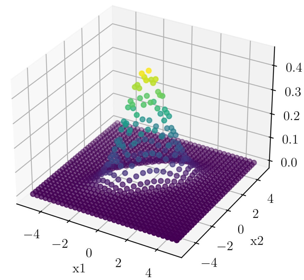
The following figure is generated in the code.
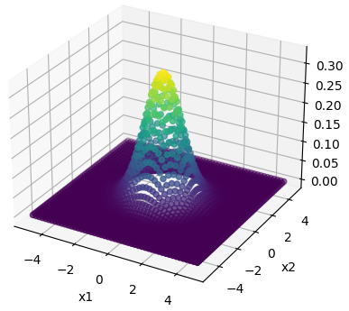
As we can see here it is centered around $(0,0)$ and having a covariance matrix of [[1, 0.0], [0.0, 1]] ranges from -5 to +5 on both dimensions.
To check our intuition lets up capture the result from the exponent term in a separate variable and use coloring to denote whether the points are of high value or low value.
Mahalanobis distance
The exponent term $\frac{1}{2}({x}-{\mu})^T{\boldsymbol\Sigma}^{-1}({x}-{\mu})$ here is known as the Mahalanobis distance and the Covariance matrix play the key role in determining which points should be amplified or attenuated.
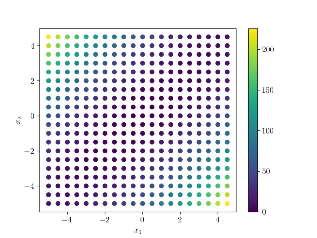
I am making a minor modification to the above code to change the covariance matrix as [[1, 0.9], [0.9, 1]] and capturing the Mahalanobis distance as a separate vector and use it to color the scatter points.
import numpy as np
import matplotlib.pyplot as plt

# set values for clean data visualization
labelsize 	= 12
width 		= 4

plt.rc('font', family ='serif')
plt.rc('text', usetex = True)
plt.rc('xtick', labelsize = labelsize)
plt.rc('ytick', labelsize = labelsize)
plt.rc('axes', labelsize = labelsize)

def myMultiVarGaussian(x1, x2, mu, Sigma):
    X = np.array((x1,x2)).T
    const = 1/(np.sqrt(((np.pi)**2)*(np.linalg.det(Sigma))))
    Sigin = np.linalg.inv(Sigma)
    MahalanobisDistance = 0.5*(np.matmul((X-mu).T, np.matmul(Sigin,(X-mu))))
    ans = const*np.exp(-1*MahalanobisDistance)
    return ans, MahalanobisDistance

mu = np.array(([0,0])).T
Sigma = np.array(([[1, 0.9], [0.9, 1]]))

X = np.arange(-5, 5, 0.5)

data = []
for x1 in X:
    for x2 in X:
        ans, MahalanobisDistance = myMultiVarGaussian(x1,x2,mu,Sigma)
        data.append([x1,x2,ans, MahalanobisDistance])

data = np.array(data)


plt.scatter(data[:,0], data[:,1], c = data[:,3])
plt.xlabel('$x_1$')
plt.ylabel('$x_2$')
plt.colorbar()
plt.savefig('BiVarHack.jpeg', dpi = 300)
plt.close()
Now if we draw the scatter plot and give the points a coloring according to the Mahalanobis distance, we can see how a high distant point (green to yellow) is giving a large distance value $k$ and taking a negative exponent of that value ($e^{-k}$) results in a low value. Whereas as a low Mahanlobis distant point (blueish) will result a negative exponent near to $e^{0}$ and high output value.
A 3d plot of the points will give a more clear picture.
For a clear visual understanding the covariance values $\sigma(x,y)$ and $\sigma(y,x)$ are changed to 0.7 here.
Conclusion
Using the code and visual representations we have inspected how the covariance matrix handles how different data points are to be amplified or attenuated. Depending upon the covariance matrix and especially the covariance values $\sigma(x_i,x_j)$, we can see how the spread can be controlled. We also inspected how the Mabanlobis distance leverages information from the covariance matrix to determine which data point to amplify or attenuate.