This article is a tutorial on the algorithm called active Learning with uncertainty Sampling.
Introduction
Availability of mass quantities of digital data and feasible computing power brought to the creation of learning algorithms. These learning algorithms have been benchmarked to perform specialized tasks such as classification, object detection, image segmentation, etc. The key assumption here is on data that is supposed to be free from human biases.
Active learning in machine learning facilitates learning by starting from a minimal set of labeled data. It follows an iterative process of choosing a new datapoint to be labeled by an oracle. The oracle is often humans in the loop who are often subject experts. Labeling dataset is often costly, time-consuming, and requires deep expertise. Active learning is a solution in such a scenario where it brings humans into the loop also.
The Active Learning Workflow
The active learning framework facilitates interaction with human experts to get the most informative data points labeled. Compared to passive learning algorithms, active learning algorithms can learn faster while maintaining minimal/feasible/economical interaction with the experts. A general workflow of active learning is depicted in the diagram below.
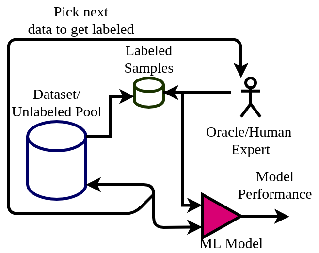
Here the algorithm starts from an unlabeled pool of data. Out of which a very small number of them is labeled. The machine learning model starts learning from this small set and picks up the next data point to get labeled. This way the ML model can pick the most informative data points for which it might have uncertainty in predicting. For a binary classifier, we can think of it as datapoints near to its initial decision boundary.
This newly picked datapoint is get labeled by human experts (also called Oracle) and added to the labeled pool. The model is again trained on the updated dataset and its performance is calculated. This process is repeated until the expected performance is achieved or the labeling cost is exhausted.
This way the algorithm gets to its peak performance with minimum data and quickly. This also solves the problem of scarcity of labeled data and efficient use of domain experts.
Code Implementation
To implement these ideas in a very basic form, let us take a problem scenario of a binary classifier. To simplify things let us create a synthetic dataset with two clusters. Cluster 1 is of class A and cluster 2 is of class B. The following figure shows the synthetic data visualized.
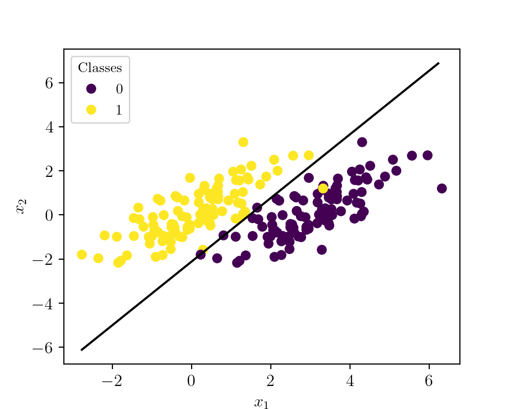
Here the yellow points denote class A and violet points represent class B. As you can see these classes overlaps each other, but still, the algorithm converges to the best fit situation. The code to create the dataset is given below.
# Import necessary libraries
import numpy as np
import pandas as pd
import matplotlib.pyplot as plt
from sklearn.metrics import accuracy_score
from sklearn.linear_model import LogisticRegression


# Set values for clean data visualization
labelsize   = 12
width       = 5
height      = 4

plt.rc('font', family ='serif')
plt.rc('text', usetex = True)
plt.rc('xtick', labelsize = labelsize)
plt.rc('ytick', labelsize = labelsize)
plt.rc('axes', labelsize = labelsize)

Class1N = 100

# Normal distributed x and y vector with mean 0 and standard deviation 1
x1 = np.random.normal(0, 1, Class1N)
x2 = np.random.normal(0, 1, Class1N)
X = np.stack((x1, x2), axis=0).T


T1 = np.asarray([[1, 0.5],[0.4,1]])
X_t1 = np.matmul(X,T1)
X_t2 = np.copy(X_t1)
X_t2[:,0]+=3


X = np.vstack((X_t1, X_t2))
y = np.append(np.ones((Class1N)),np.zeros((Class1N)))
X_t = np.column_stack((X, y))
np.random.shuffle(X_t)


data = pd.DataFrame(X_t, columns = ['x1','x2','label'])
data.to_csv('./SynData/data.csv')

features = data.values[:,:-1]
labels = data.values[:,-1]


LRC = LogisticRegression()
LRC.fit(features, labels)


# Retrieve the model parameters.
b = LRC.intercept_[0]
w1, w2 = LRC.coef_.T

# Calculate the intercept and gradient of the decision boundary.
c = -b/w2
m = -w1/w2


u = np.arange(np.min(X_t[:,0]), np.max(X_t[:,0]),0.5)
v = m*u+c

fig1, ax = plt.subplots()
plt.plot(u, v, c='k')
scatter = plt.scatter(features[:,0], features[:,1], c=labels)
legend1 = ax.legend(*scatter.legend_elements(),
                    loc="upper left", title="Classes")
plt.xlabel('$x_1$')
plt.ylabel('$x_2$')
plt.show()
fig1.set_size_inches(width, height)
fig1.savefig('./Graphs/DataSet.png', dpi=200)
The code also saves the synthetic data as a CSV file. Now let us take a moment to design some experiments to evaluate the performance of the active learning algorithm. I chose logistic regression as a classifier. The line shows its classification boundary if all data points were available as labeled.
Experiment Design
All of the experiments are done 20 times and the results are averaged. The dataset is split into the train (70 samples) and test (30 samples). The classifier accuracy is always calculated on the test data.
Experiment 1: Iterative learning in batches. The classifier starts with 10 labeled data points. After each iteration, it randomly picks 10 more from the pool and adds them to the labeled pool. The model is trained on the new labeled set and accuracy is computed against the test dataset.
Experiment 2: Iterative learning random pick. The classifier starts with 10 labeled data points. After each iteration, it picks 1 more from the pool randomly and adds it to the labeled pool. The model is trained on the new labeled set and accuracy is computed against the test dataset.
Experiment 3: Active learning with Uncertainty Sampling. The classifier starts with 10 labeled data points. After each iteration, it picks 1 more from the pool based on uncertainty sampling and adds it to the labeled pool. The model is trained on the new labeled set and accuracy is computed against the test dataset.
The implementation code for all three experiments is given below.
Experiment 1 Code:
# Import necessary libraries
import numpy as np
import pandas as pd
from tqdm import tqdm
from numpy import save
import matplotlib.pyplot as plt
from sklearn.model_selection import train_test_split
from sklearn.metrics import accuracy_score
from sklearn.linear_model import LogisticRegression


# Set values for clean data visualization
labelsize   = 12
width       = 4
height      = 4

plt.rc('font', family ='serif')
plt.rc('text', usetex = True)
plt.rc('xtick', labelsize = labelsize)
plt.rc('ytick', labelsize = labelsize)
plt.rc('axes', labelsize = labelsize)


data = pd.read_csv('./SynData/data.csv').values

y = data[:,-1]
X = data[:,:-1]


numDataTotal = 140
labeledPoolN = 10
batchSz = 10

nAccs = (numDataTotal-labeledPoolN)//batchSz


monteN = 200

def computeAccuracy(dataL):
    y_trainC = dataL[:,-1]
    X_trainC = dataL[:,1:-1]
    LRC = LogisticRegression()
    LRC.fit(X_trainC, y_trainC)
    y_pred = LRC.predict(X_test[:,1:])
    Acc = accuracy_score(y_test, y_pred)
    return np.array([[Acc]]), LRC


def getBatch(dataPool, batchSz):
    dataBatch = dataPool[np.random.choice(dataPool.shape[0], batchSz, replace=False), :]
    remIdx = np.isin(dataPool[:,0], dataBatch[:,0], invert=True)
    dataPool = dataPool[remIdx]

    return dataBatch, dataPool


accuracySmooth = []

X_train, X_test, y_train, y_test = train_test_split(X, y, test_size=0.30,random_state=5)


for monte in tqdm(range(monteN)):

    dataPool = np.hstack((X_train, np.atleast_2d(y_train).T))

    dataPoolL = dataPool[np.random.choice(dataPool.shape[0], labeledPoolN, replace=False), :]

    remIdx = np.isin(dataPool[:,0], dataPoolL[:,0], invert=True)

    dataPool = dataPool[remIdx]

    AccuracyRes = np.empty((0,1), float)

    accStart, cModel = computeAccuracy(dataPoolL)

    AccuracyRes = np.append(AccuracyRes, accStart, axis=0)

    for i in range(nAccs):
        dataBatch, dataPool = getBatch(dataPool, batchSz)
        dataPoolL = np.vstack((dataPoolL, dataBatch))
        cAcc, cModel = computeAccuracy(dataPoolL)
        AccuracyRes = np.append(AccuracyRes, cAcc, axis=0)
    accuracySmooth.append(AccuracyRes)

accuracySmooth = np.asarray(accuracySmooth)
accuracySmooth = np.mean(accuracySmooth, axis=0)


fig1 = plt.figure()
plt.plot([x for x in range(labeledPoolN, numDataTotal+1, batchSz)], accuracySmooth)
plt.xlabel('Number of samples')
plt.ylabel('accuracy')
plt.show()


graphData = np.array(([x for x in range(labeledPoolN, numDataTotal+1, batchSz)], accuracySmooth.flatten()))
save('./Graphs/Active_Learning_Batch.npy', graphData)
Experiment 2 Code:
# Import necessary libraries
import numpy as np
import pandas as pd
from tqdm import tqdm
from numpy import save
import matplotlib.pyplot as plt
from sklearn.model_selection import train_test_split
from sklearn.metrics import accuracy_score
from sklearn.linear_model import LogisticRegression


# Set values for clean data visualization
labelsize   = 12
width       = 4
height      = 4

plt.rc('font', family ='serif')
plt.rc('text', usetex = True)
plt.rc('xtick', labelsize = labelsize)
plt.rc('ytick', labelsize = labelsize)
plt.rc('axes', labelsize = labelsize)


data = pd.read_csv('./SynData/data.csv').values

y = data[:,-1]
X = data[:,:-1]


numDataTotal = 140
labeledPoolN = 10
batchSz = 1

nAccs = (numDataTotal-labeledPoolN)//batchSz


monteN = 200

def computeAccuracy(dataL):
    y_trainC = dataL[:,-1]
    X_trainC = dataL[:,1:-1]
    LRC = LogisticRegression()
    LRC.fit(X_trainC, y_trainC)
    y_pred = LRC.predict(X_test[:,1:])
    Acc = accuracy_score(y_test, y_pred)
    return np.array([[Acc]]), LRC


def getBatch(dataPool, batchSz):
    dataBatch = dataPool[np.random.choice(dataPool.shape[0], batchSz, replace=False), :]
    remIdx = np.isin(dataPool[:,0], dataBatch[:,0], invert=True)
    dataPool = dataPool[remIdx]

    return dataBatch, dataPool


accuracySmooth = []

X_train, X_test, y_train, y_test = train_test_split(X, y, test_size=0.30,random_state=5)


for monte in tqdm(range(monteN)):

    dataPool = np.hstack((X_train, np.atleast_2d(y_train).T))

    dataPoolL = dataPool[np.random.choice(dataPool.shape[0], labeledPoolN, replace=False), :]

    remIdx = np.isin(dataPool[:,0], dataPoolL[:,0], invert=True)

    dataPool = dataPool[remIdx]

    AccuracyRes = np.empty((0,1), float)

    accStart, cModel = computeAccuracy(dataPoolL)

    AccuracyRes = np.append(AccuracyRes, accStart, axis=0)

    for i in range(nAccs):
        dataBatch, dataPool = getBatch(dataPool, batchSz)
        dataPoolL = np.vstack((dataPoolL, dataBatch))
        cAcc, cModel = computeAccuracy(dataPoolL)
        AccuracyRes = np.append(AccuracyRes, cAcc, axis=0)
    accuracySmooth.append(AccuracyRes)

accuracySmooth = np.asarray(accuracySmooth)
accuracySmooth = np.mean(accuracySmooth, axis=0)


fig1 = plt.figure()
plt.plot([x for x in range(labeledPoolN, numDataTotal+1, batchSz)], accuracySmooth)
plt.xlabel('Number of samples')
plt.ylabel('accuracy')
plt.show()


graphData = np.array(([x for x in range(labeledPoolN, numDataTotal+1, batchSz)], accuracySmooth.flatten()))
save('./Graphs/Active_Learning_Iterative.npy', graphData)
Experiment 3 Code:
# Import necessary libraries
import numpy as np
import pandas as pd
from tqdm import tqdm
from numpy import save
import matplotlib.pyplot as plt
from sklearn.model_selection import train_test_split
from sklearn.metrics import accuracy_score
from sklearn.linear_model import LogisticRegression


# Set values for clean data visualization
labelsize   = 12
width       = 4
height      = 4

plt.rc('font', family ='serif')
plt.rc('text', usetex = True)
plt.rc('xtick', labelsize = labelsize)
plt.rc('ytick', labelsize = labelsize)
plt.rc('axes', labelsize = labelsize)


data = pd.read_csv('./SynData/data.csv').values

y = data[:,-1]
X = data[:,:-1]


numDataTotal = 140
labeledPoolN = 10
nAccs = numDataTotal-labeledPoolN+1

monteN = 200


def computeAccuracy(dataL):
    y_trainC = dataL[:,-1]
    X_trainC = dataL[:,1:-1]
    LRC = LogisticRegression()
    LRC.fit(X_trainC, y_trainC)
    y_pred = LRC.predict(X_test[:,1:])
    Acc = accuracy_score(y_test, y_pred)
    return np.array([[Acc]]), LRC


def getBestDpoint(dataPool, cModel):
    entropyVector = np.empty((0,2), float)
    for row in dataPool:
        trow = row[1:-1].reshape(1,-1)
        logP = cModel.predict_log_proba(trow)[0]
        prob = cModel.predict_proba(trow)[0]
        entropy = -1*np.sum(np.multiply(prob, logP))
        entropyVector = np.append(entropyVector, np.array([[row[0], entropy]]), axis=0)
    imax = np.argmax(entropyVector[:,1])
    indexUncertain = entropyVector[imax][0]
    bestDataPoint = dataPool[dataPool[:,0]==indexUncertain, :]
    return bestDataPoint


accuracySmooth = []

X_train, X_test, y_train, y_test = train_test_split(X, y, test_size=0.30,random_state=5)

for monte in tqdm(range(monteN)):

    dataPool = np.hstack((X_train, np.atleast_2d(y_train).T))

    dataPoolL = dataPool[np.random.choice(dataPool.shape[0], labeledPoolN, replace=False), :]

    remIdx = np.isin(dataPool[:,0], dataPoolL[:,0], invert=True)

    dataPool = dataPool[remIdx]

    AccuracyRes = np.empty((0,1), float)

    accStart, cModel = computeAccuracy(dataPoolL)

    AccuracyRes = np.append(AccuracyRes, accStart, axis=0)

    for i in range(numDataTotal-labeledPoolN):
        dataPointUncertain = getBestDpoint(dataPool, cModel)
        dataPoolL = np.vstack((dataPoolL, dataPointUncertain))
        remIdx2 = np.isin(dataPool[:,0], dataPoolL[:,0], invert=True)
        dataPool = dataPool[remIdx2]
        cAcc, cModel = computeAccuracy(dataPoolL)
        AccuracyRes = np.append(AccuracyRes, cAcc, axis=0)
    accuracySmooth.append(AccuracyRes)

accuracySmooth = np.asarray(accuracySmooth)
accuracySmooth = np.mean(accuracySmooth, axis=0)


fig = plt.figure()
plt.plot([x for x in range(labeledPoolN, nAccs+labeledPoolN)], accuracySmooth)
plt.xlabel('Number of samples')
plt.ylabel('accuracy')
plt.show()


graphData = np.array(([x for x in range(labeledPoolN, nAccs+labeledPoolN)], accuracySmooth.flatten()))
save('./Graphs/Active_Learning_Uncertainity_Sampling.npy', graphData)
Experiment 3 Animation
The following video shows what happens to the classifier decision boundary, labeled samples, accuracy, and entropy at every iteration for a single run. The visual representation of the classifier is shown on right and the accuracy and entropy values are shown on left. The algorithm picks unlabeled samples with higher entropy which are actually the ones near to the decision boundary to get labeled. As it starts sampling away from decision boundary the entropy starts to drop off quickly.
All the codes will experiment around 200 times and averages out the accuracy curves. The performance curve will be the number of labeled data points vs. accuracy. I have saved the results from each program as NumPy files for later use. Once we run all these experiments we can plot the graphs in one plot. The following code does the plotting.
# import some libraries
import numpy as np
import matplotlib.pyplot as plt

# set values for clean data visualization
labelsize   = 12
width       = 5
height      = 4

plt.rc('font', family ='serif')
plt.rc('text', usetex = True)
plt.rc('xtick', labelsize = labelsize)
plt.rc('ytick', labelsize = labelsize)
plt.rc('axes', labelsize = labelsize)


data1 = np.load('Active_Learning_Iterative.npy')
data2 = np.load('Active_Learning_Batch.npy')
data3 = np.load('Active_Learning_Uncertainity_Sampling.npy')

# print(data1.shape)
# print(data2.shape)
# print(data3.shape)
# print(data4.shape)

fig, ax = plt.subplots()
fig.subplots_adjust(left=.2, bottom=.2, right=.97, top=.90)
# plt.xlim([0, 200])

# plt.axhline(y=1, color='r', linestyle='--', label='Peak Performance')
plt.plot(data1[0],data1[1], label ='Iterative')
plt.plot(data2[0],data2[1], label ='Batch')
plt.plot(data3[0],data3[1], label ='AL US')

# ax.legend(bbox_to_anchor=(1, 0), loc='lower right')
ax.legend(loc='lower right')

plt.xlabel('Number of samples')
plt.ylabel('Accuracy')
plt.show()

fig.set_size_inches(width, height)
fig.savefig('Active_Learning_Exp_Results.png', dpi=200)
plt.close()
Results
Now let us check the results from each experiment. The following graph shows the results.
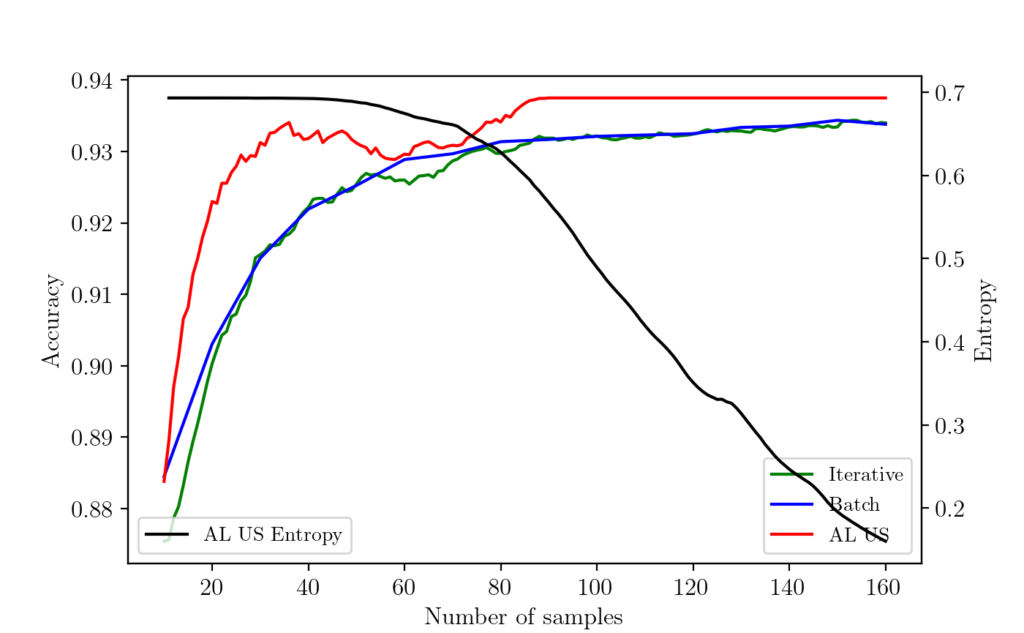
As you can see here, the active learning algorithm with uncertainty sampling learns much faster and achieves the peak performance with a minimum number of samples. The batch and iterative sampling learn as it receives more labeled datapoint.
Concluding Remarks
This article demostrated a very basic implementaion of active learning algorithm with uncertainity sampling. The performance of active learner is compared agains other type of interative methods.