Overview
Materials science is a field of study that involves the research and discovery of new materials and its functional properties for applications in electronic storage devices, biomedical instrumentation, telecommunication equipment etc. The applications of material science spans from designing of products by exploiting its material properties to the manufacture of products which can contribute to the advancement of technology.
The perovskite materials open up a receptive scope in material science research owing to its simple structure and diverse scope to be exploited in terms of modulated material and physical properties. The manipulations in the properties can be achieved through the lattice distortion. The lattice distortions induce crystal structure transformations from its ideal cubic structure to other low symmetry structures and hence the material properties change due to structure-property relations.
The perovskite structure can be understood from the general formula $ABO_3$. Wherein the A-site is occupied by a large size cation surrounded by 12 oxygen anions and the B-Site consists of a small size cation at the center of an oxygen Octahedra as shown in Fig.1. The structural modifications in perovskite structure have diverse applications in spintronics, magnetism and other areas of physics and material science.
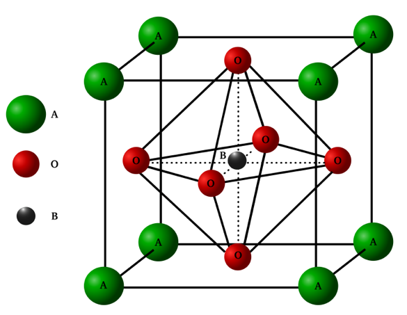
Fig. 1 Schematic of ideal Perovskite structure
When we combine elements to get perovskite structure, the electronegativity helps the functional groups to attract each other to form a stable compound. Electronegativity of an element is a relative parameter which varies in relation with the other elements to which it is bound or interacts. The difference in electronegativity with radius ($\Delta$ENR) has considerable importance to interpret the lattice distortion undergone by a compound and the associated changes in crystal structure. Hence it is of utmost importance to extract its value after it forms the compound from measurable physical parameters instead of calculating it from estimated electronegativity of individual constituent elements.
This case study demonstrate and explains the various stages to predict the $\Delta$ENR of perovskites from measurable structural features such as radius of the element A at 12 coordination, radius of A at 6 coordination, bond length of A-O pair, bond length of B-O pair, Goldschmidt tolerance factor, new tolerance factor, and octahedral factor as well as it explores the impact of valence state of heavy atom on A-site such as valence A-1, valence A-2 and valence A-3.
Dataset
The dataset used for this project is published in Mendeley data named as “Data for: Crystal structure classification in ABO3 perovskites via machine learning” by Behera, Poonawalla et. al., Mendeley Data, V1, doi: 10.17632/dfsf6n6g7y.1. This data is produced as supporting data for a research paper the authors published in the journal of computational materials science.
Part 1 of the dataset contains a list of all 5329 ABO3 perovskite-type oxides in Microsoft Excel Worksheet format and part 2 of the dataset, which is used for this case study contains a list of all 675 ABO3 perovskite-type oxides in Microsoft Excel Worksheet format.
Performance Metric and Primary Performance Metric
Here in this case study, the objective is to predict the value of $\Delta$ENR from structural features. Hence the problem is framed as a regression problem in machine learning. The performance metrics considered are R2-score and Mean Squared Error (MSE). The R2-score tells how better the model will be compared to a simple model which predicts the mean value of the output variable. The value of R2-score can range from 0 to 1 and any value above 0.7 can be considered as a good indication that the model is predicting target value well. So, the primary performance metric will be R2-score.
The secondary performance metric is MSE value. This tells how much is the average of squared errors (i.e., the mean of squared values of difference between actual target values and predicted values). Hence MSE will be also used to monitor the model performance.
Research Approaches Referred
1. Behera, Poonawalla et al. “Crystal structure classification in $ABO_3$ perovskite via machine learning” Comput.Mater.Sci. 188 (2021),110191.
URL: https://doi.org/10.1016/j.commatsci.2020.110191
In this paper, the authors have done crystal structure classification of perovskites into their respective crystal systems of cubic, rhombohedral, orthorhombic and tetragonal. They have used the data set of 5329 Perovskite compounds and successfully classified 675 compounds. The required multiclass classification was performed using the Light gradient boosting machine (GBM) model. They have used features such as valence state, radius, electronegativity, tolerance factor etc. to do the classification task. The Light GBM model shows an accuracy of 80.3 %. Hence, they have presented the model as an inexpensive and fast computational method to classify perovskite compounds into their corresponding crystal structure system.
2. Li, Dan et al. “Computational Screening of New Perovskite Materials Using Transfer Learning and Deep Learning” App.Sci.9 (2019), 5510
URL: https://doi.org/10.3390/app9245510
In this paper, the authors successfully executed computational prediction of novel perovskite materials for potential applications. They employed a transfer-based learning approach enabled with physics informed structural and elemental descriptors. They could predict the formation energy with sufficient precision for a large number of materials from the structural information available. They have extended their studies by conducting experiments with reference to the predicted values. The experiments validate the superior performance of their transfer learning model as compared to the baseline models. The article describes this gradient boosting regressor model (transfer learning model) as a suitable screening out model to filter out promising perovskite materials out of the 21316 hypothetical perovskite structures.
First Cut Approach
The initial steps followed in this case study consist of examining the data for the number of data points, features, and target variables, analyse whether the data is numerical or categorical, etc. Only relevant features are considered for further data processing. Any column omission is justified with possible reasoning. Further the selected features are checked for missing values and basic descriptive statistics.
The next step executed is the detailed Exploratory Data Analysis (EDA) of the data available. EDA is performed extensively to determine the correlation of features to target variable, data distribution, and statistical significance. The EDA is supported with scientific plots to illustrate the findings. The plots includes correlation plots, density plots, scatter plots etc.
In the modeling part, after train test split and 5-fold cross validation, multiple classical regression models are tried out such as lasso regression, support vector regression, random forest regressor, Bayesian ridge based regressor and gradient boosting regressor. The performance metrics of each of these models are evaluated and used further to select the final model.
Since the computational prediction of $\Delta$ENR from structural features is novel to the best of my knowledge, the potential use case and workflow is discussed briefly.
Business Constraints
The primary business constraint is the availability of experimental data. Data corresponding to the relevant features will be able to generate only from sophisticated experimental physics labs. The cost of such experiments and equipment required need to be considered from a product standpoint.
Another constraint is further use cases such as perovskite structure prediction from $\Delta$ENR values need to be validated by human supervision. This puts a dependency of domain experts for such applications.
Exploratory Data Analysis
The dataset is loaded for exploratory data analysis followed by the import of necessary libraries. As a primary data pre-processing step, the irrelevant columns are dropped. The code snippet used for the aforementioned task is as below,
import pandas as pd
from tqdm import tqdm
import seaborn as sns
import matplotlib.pyplot as plt
from scipy.stats import zscore
data = pd.read_csv('./data/file_2.csv')
data = data.drop(['S.No'], axis=1)
In addition, the column names are printed to understand the existed features in the dataset.
The number of cations in the A site and B site are visualized using bar plots in order to get an overview of prominent cations at these sites in perovskites considered for this case study.
The code snippet is shared along with the corresponding figures (Fig. 2 and Fig. 3).
Code to understand the number of cations in A site in the entire dataset analysed,
fig, ax = plt.subplots(figsize=(8, 10))
A.value_counts().plot(kind = 'barh')
for container in ax.containers:
ax.bar_label(container)
plt.xlabel('Count')
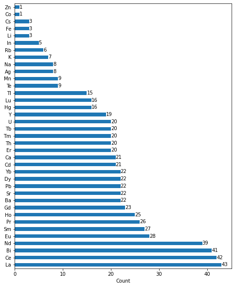
Fig. 2 Bar plot of Cations in A site of the dataset
Code to understand the number of cations in B site in the entire dataset analysed,
B = data['B']
fig, ax = plt.subplots(figsize=(8, 10))
B.value_counts().plot(kind = 'barh')
for container in ax.containers:
ax.bar_label(container)
plt.xlabel('Count')
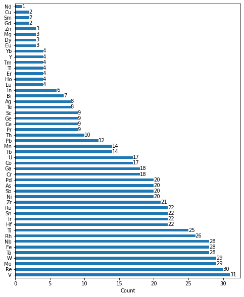
Fig. 3 Bar plot of Cations in B site of the dataset
The compounds which undergone distortion from the ideal perovskite structure among the entire compounds used in these case study are further analyzed using the bar plot. The visualization revealed, 261 compounds crystallized to the high symmetry cubic crystal structure once form the compound. The remaining compounds crystallized to low symmetry crystal structures such as orthorhombic, tetragonal and rhombohedral.
The code snippet to understand the number of distorted compounds to low symmetry crystal structure and the corresponding visualization ( Fig. 4) is as follows,
structure_type = data['Lowest distortion']
fig, ax = plt.subplots(figsize=(6, 5))
structure_type.value_counts().plot(kind = 'barh')
for container in ax.containers:
ax.bar_label(container)
plt.xlabel('Count')
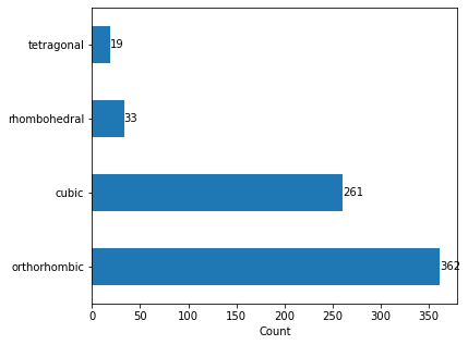
Fig. 4 Visualization of number of compounds undergone crystal structure distortion
The valence state of an element determines the ability of an element to combine with other elements. The electronegativity of elements increases with valence state. The valance state of element at A and element at B are categorical values and so plotted it using bar plot for further analysis of its effect on the target variable.
The code snippet and the corresponding figures ( Fig. 5 and Fig. 6) are included below,
va = data['v(A)']
fig, ax = plt.subplots(figsize=(6, 5))
va.value_counts().plot(kind = 'barh')
for container in ax.containers:
ax.bar_label(container)
plt.xlabel('Count')
plt.ylabel('v(A)')

Fig. 5 Bar Plot of valence state of elements at A site
vb = data['v(B)']
fig, ax = plt.subplots(figsize=(6, 5))
vb.value_counts().plot(kind = 'barh')
for container in ax.containers:
ax.bar_label(container)
plt.xlabel('Count')
plt.ylabel('v(B)')
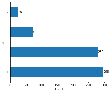
Fig. 6 Bar Plot of valence state of elements at B site
In order to understand the impact of features on the target variable, it is important to analyse its distribution. Here, the features under consideration are radius of element A at 12 coordination as well as 6 coordination, radius of B at 6 coordination, Electronegativity of elements at A and B sites, bond length of A-O pair and B-O pair, estimated electronegativity difference with radius, Goldschmidt tolerance factor, new tolerance factor and Octahedral factor. The statistical distribution of relevant features are analysed in detail. Among these features, the distribution of estimated electronegativity difference with radius is analysed for the comparison of the predicted electronegativity difference with radius with the estimated value.
Analysis of Missing Values
The data is examined for missing values and visualized using heatmap in seaborn library. The code snippet and output image (Fig. 7) is shown below. As there are no missing values in any of the columns, we get a single colour image as heatmap output.
fig, ax = plt.subplots( figsize = (10, 6))
sns.heatmap(combined_table.isnull())
ax.set_title('Missing values in data')
plt.show()
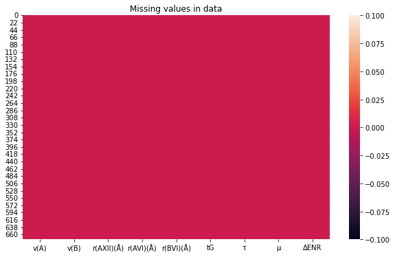
Fig. 7 Heatmap of missing values
Correlation between features
Most of the features are moderately correlated with each other. The code snippet and histogram ( Fig. 8 ) of the same is shown below.
X_matrix = X.corr().values
plt.hist(X_matrix.flatten(),10)
plt.xlabel('Pearson correlation coefficient bw features')
plt.ylabel('Count')
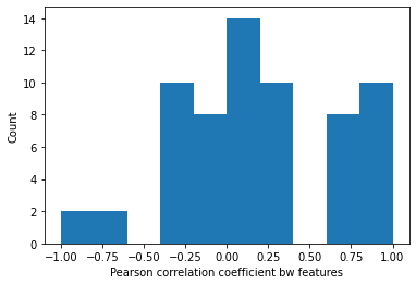
Fig. 8 Correlation between features
The following figure ( Fig. 9) shows correlation between features as a heatmap.
fig, axs = plt.subplots(figsize = (8, 6))
sns.heatmap(X.corr())
plt.title('Feature correlation heatmap')
plt.show()
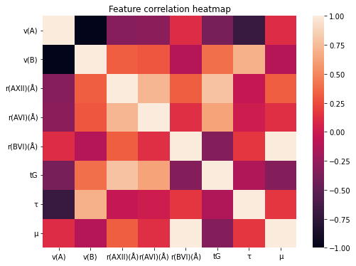
Fig. 9 Heatmap of correlation among features
Violin Plot of Features Used
The violin plot (Fig. 10) of features used for the modeling is shown below. The violin plot shows the quantile values, median and distribution in a single plot.
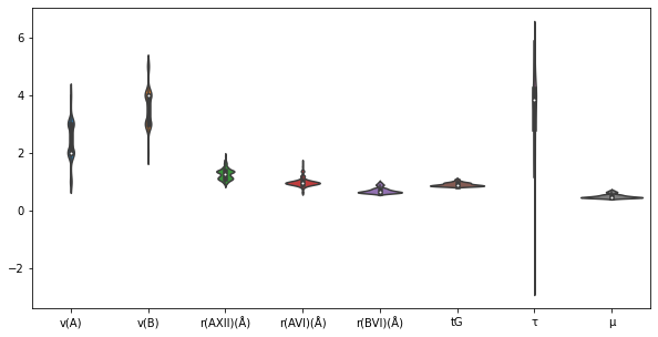
Fig. 10 Violin plot of features with considerable significance
Outlier heatmap
The outliers of the features, where |zscore|>3, if any is visualized ( Fig. 11) using heatmap shown below. Four out of eight features are having outlier points with z-score above or below 3 standard deviations.
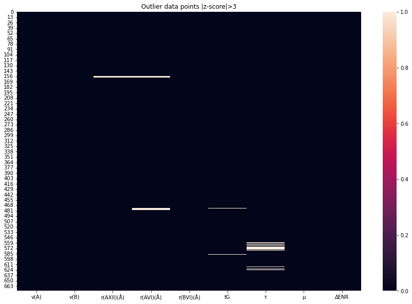
Fig. 11 Heatmap of outliers of features
Inferences from EDA
EDA has been performed to visualise the features and to identify the correlation among features of considerable importance on target variable. The irrelevant column such as serial number has been dropped The target variable $\Delta$ENR is identified as a continuous numerical variable, hence the problem is framed as a machine learning regression task. In the dataset, there are 675 datapoints and 19 columns including target variable in the original data. Six columns are categorical (compound name, cation in A site, cation in B site, crystal structure, valance A, and valance B) and rest of them are numerical. The crystal structure to which the 675 perovskites under study are tetragonal, rhombohedral, cubic and orthorhombic. EDA confirms that there are no missing values in the dataset.
The Pearson correlation, which is a measure of strength and direction to which two features depends on each other is dispersed across +1 and -1. There are few outlier points (z-score>3 or z-score<-3) for radius of element at A site with 12 coordination as well as 6 coordination, Goldschmidt tolerance factor and new tolerance factor.
Modeling to predict $\Delta$ENR of Perovskites
In the modeling part of this case study, following regression methods are used such as support vector regression, Bayesian ridge regressor, lasso regressor, random forest regressor and gradient boosting regressor.
Hyperparameter tuning
The hyperparameter tuning is performed using Gridsearchcv module in scikit-learn. The parameters selected to tune in each model is as follows.
# Lasso regression
ls_params = {'alpha':[0.02, 0.025, 0.03]}

# Random forest
rf_params = {'n_estimators': [200, 500],
'max_features': ['sqrt', 'log2'],
'max_depth' : [4,6,8]}

# Support vector regression
svr_params = {'kernel': ['rbf'],
'gamma': [0.01, 0.1, 0.5],
'C': [1, 10, 1000]}

# Bayesian ridge regression
bay_params = {'alpha_init':[1, 1.5, 1.9],
'lambda_init': [1e-2, 1e-5, 1e-9]}

# Gradient boosting regression
gb_params = {'learning_rate': [0.01,0.03],
'subsample' : [0.5, 0.1],
'n_estimators' : [100,500],
'max_depth' : [4,8,10]}
The function to do hyperparameter tuning using GridsearchCV is given below.
def grid_search_train(model_name, model, model_params, X_train, y_train):
    grid_model = GridSearchCV(estimator=model, param_grid=model_params, cv=5)
    grid_model.fit(X_train, y_train)
    print('\nBest params of {} model are:'.format(model_name))
    print(grid_model.best_params_)
    return grid_model
Feature Engineering
A new feature has been derived by taking the difference of electronegativity of element at A site and B site.
X['feat_3'] = data['EN(A)']-data['EN(B)']
This new feature was found to improve the regression output slightly. Other methods such as Fourier transform and algebraic transformation of multiple features were tried out and found to be not contributing to improve the prediction results.
The performance of the models are assessed from R2 score and mean square error and displayed in the pretty table (Table. 1). Inorder to avoid overfitting of the models, 5-fold cross validation was carried prior to performance metric calculation.
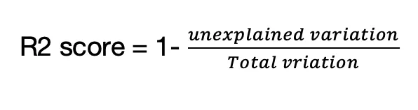
R2 score is a statistical measure to quantify the variance of dependent features which are in relationship with features in a regression model,
The equation to calulate R2 score is,
The mean square error (MSE) is another performance metric use in regression models. The MSE tells how close a regression line is to the data points.
MSE can be understood from the equation,
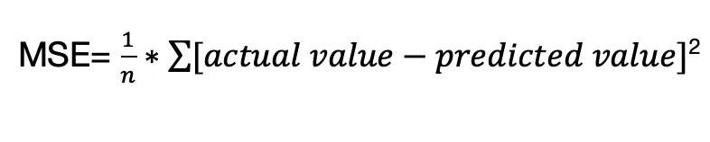
Where n is the size of the sample
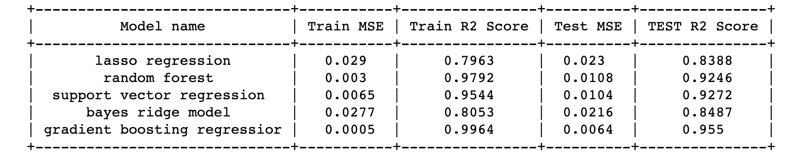
Table 1. Performance metrics of different models
Summary
The observations of this case study are summarised as,
- Gradient Boosting Regressor is the best performing model with test MSE of 0.0064 and test R2 score of 0.9550
- All models are having a reasonable good test R2 score on or above 0.8
- Performing standard scaling improves performance of lasso regression significantly and minor improvements for other models also
- Adding absolute Fourier transform values or algebraic transformations to features does not improve model performance
- Including EN(A) and EN(B) features improve all model’s R2 score
Article originally published in medium