Overview
Birds are an incredibly diverse group of animals found all over the Earth. With over 10,000 known species, they come in all shapes, sizes, and colours, and they play a vital role in maintaining the delicate balance of ecosystems around the world.
One of the most important roles that birds play is that of pollination. Many species of birds feed on nectar and pollen from flowers, and as they move from one flower to the next, they transfer pollen from one plant to another. This helps to ensure that plants can reproduce and create new generations of offspring. Birds are also important seed dispersers. As they fly around, they eat fruits and berries, and the seeds pass through their digestive tracts unharmed. When the birds defecate, the seeds are deposited in a new location, which can help the plant species to spread and colonize new areas.
However, birds are facing numerous threats, including habitat loss, climate change, and pollution. Many bird populations are declining, and some species are at risk of extinction. This is not only a tragedy for the birds themselves but also for the ecosystems they inhabit and the humans who rely on those ecosystems for their own well-being.
Kerala is home to a diverse array of bird species, with over 500 species recorded in the state. From the wetlands and backwaters to the Western Ghats, the varied landscapes of Kerala provide habitats for a range of birds, including both resident and migratory species.
One of the most fascinating aspects of birding in Kerala is the rich variety of bird songs that can be heard throughout the state. Bird song identification and monitoring are also important for conservation efforts in Kerala. By recording and identifying bird songs, researchers can gather data on the distribution and abundance of different bird species, which can inform conservation policies and management strategies. For example, by tracking changes in bird populations over time, scientists can identify areas where habitat restoration or protection may be needed.
In addition, bird song monitoring can also provide important insights into the impacts of climate change and other environmental factors on bird populations. Changes in bird song patterns or the absence of certain bird species from an area can be an early warning sign of ecological disturbances or habitat degradation.
Automated bird song identification and monitoring using machine learning/deep learning has the potential to revolutionise the way we study and conserve bird populations. Deep learning algorithms can be trained to recognise patterns in bird songs, allowing for accurate and efficient identification of different species.
The process of automated bird song identification typically involves collecting audio recordings of bird songs and using specialized software to extract features such as pitch, tempo, and frequency. These features are then used to train deep learning algorithms, which can learn to recognize the unique characteristics of different bird species.
One advantage of automated bird song identification is that it allows for large amounts of data to be collected and analyzed quickly and efficiently. This is particularly useful for monitoring bird populations over time, as it allows for changes in bird distribution and abundance to be tracked and analyzed on a large scale.
Automated bird song identification can also help to overcome some of the limitations of human-based bird identification. For example, bird songs can be highly complex, and some species have songs that are difficult for even experienced birdwatchers to differentiate. By contrast, machine learning algorithms can be trained to recognize even subtle differences between bird songs, which can improve the accuracy and reliability of bird population monitoring.
Despite its potential benefits, automated bird song identification is not without its challenges. One significant challenge is the need for high-quality audio recordings, which can be difficult to obtain in certain environments. In addition, different bird species may have overlapping songs or may change their songs over time, which can make accurate identification more difficult.
Dataset
The taxonomy of birds in Kerala is documented in the recent bird atlas survey titled “An atlas of the birds of Kerala” by Praveen J & PO Nameer (available online). The bird song recordings are freely available to download from the websites https://indianbirdsong.org/ and https://xeno-canto.org/.
A total number of 382 species of birds was recorded during the Bird Atlas survey in Kerala. This comes to more than 70% of the total species of birds ever recorded in Kerala. Out of the 63 species of birds belonging to the threatened category of International Union for Conservation of Nature (IUCN) known from Kerala (as on September 2020), 35 species were encountered during the Atlas survey.
In this case study, I am trying to create deep learning based classifiers which can identify these 35 endangered bird species from their song recordings. Once the classifier is built and deployed as a REST API, web app or smartphone app, it has the potential to be used by anyone interested to detect or monitor the population of these endangered species.
Performance Metrics and Primary Performance Metric
This problem is a multi-class classification (35 classes) problem. The primary performance metric is micro F1-score. Along with its accuracy, micro-averaged Precision, Recall, and F1 scores of each class are also monitored.
Research-Papers/Solutions/Architectures/Kernels
N. A. and R. Rajan, “Deep Learning-based Automatic Bird Species Identification from Isolated Recordings,” 2021 8th International Conference on Smart Computing and Communications (ICSCC), Kochi, Kerala, India, 2021, pp. 252–256, doi: 10.1109/ICSCC51209.2021.9528234.
This research work deals with the task of identifying multiple bird species from audio recordings. Deep Convolutional Neural Network (Deep CNN), VGG-16 model has been used to train and classify audio recordings into 10 different species. The database used was the Xeno-canto bird sound database. As features Mel-spectrograms and Mel Frequency Cepstral Coefficients are used. They report the classification performance of an average F1-score of 0.65. To improve the results the authors have used a data augmentation technique called SpecAugment.
Praveen, J., Nameer, P. O., Jha, A., Aravind, A., Dilip, K. G., Karuthedathu, D., … & Rowther, B. E. (2022). Kerala Bird Atlas 2015–2020: features, outcomes and implications of a citizen-science project. Current Science, 122(3), 298.
This paper gives details about how the bird atlas survey was carried out, its data collection and sampling methods, data filtering, limitations, and recommendations. After eliminating nocturnal and pelagic species, data from 361 species were analyzed.
First Cut Approach
The first step followed is simple data analysis and Exploratory Data Analysis of the bird songs. Both the time domain and frequency domain (Spectrograms) of various sample recordings are plotted. Also, these sounds are played using audio playback features so that the user gets a feel of the bird species and its unique call. As a first model, spectrograms of these bird songs are generated as features and an initial model is constructed. An initial 35-class CNN model is constructed and trained. The performance of this model is evaluated on test data using 5-fold cross-validation.
As the next step, Mel-Frequency Cepstral Coefficients are generated as features from the audio. The performance of this second model is evaluated. Rest of the improvements such as more feature engineering, hyperparameter tuning, and data augmentation, transfer learning with other image base models are performed as per the requirements identified on various stages.
Business Constraints
The primary business constraint/challenge here is the noise in the audio recording. There is an alternate noise interventions such as other mammalian sounds, noise due to human intervention, and noise pollution. Identifying overlapping bird calls is also be another challenge encountered. The large-scale full potential application of this project requires crowd-source efforts from citizens in various regions in Kerala. Continuous monitoring requires recording devices with longer power backup which can be kept as automated monitoring devices in ecologically sensitive areas. Old smartphones can be repurposed for this and it can be made to sync the data (time, GPS location, species identified, bird call, etc.) automatically to a central database.
Exploratory Data Analysis
After the import of necessary libraries, the dataset is loaded for exploratory data analysis (EDA). The basic dataset information are extracted as a preliminary data pre-processing step. I have focussed on 25 species for which recordings are available out of the 35 endangered bird species from Kerala bird atlas
The code snipped for these steps are as follows,
import re
import librosa
import warnings
import numpy as np
import pandas as pd
from os import listdir
from tqdm import tqdm
import seaborn as sns
from os.path import join
import IPython.display as ipd
import matplotlib.pyplot as plt
warnings.filterwarnings('ignore')
from sklearn.manifold import TSNE
from sklearn.decomposition import PCA
from sklearn.preprocessing import LabelEncoder
endangerd_species_path = '/kaggle/input/endagerd-bird-species-of-kerala/endagered_bird_species_of_kerala.csv'
audio_path = '/kaggle/input/kerala-endangered-bird-species-audio/'
endangered_species = pd.read_csv(endangerd_species_path)
audio_list = listdir(audio_path)
endangered_species['scientific_name'] = endangered_species['scientific_name'].str.lower()
endangered_species_kerala = list(set(endangered_species['scientific_name'].tolist()))
endangered_species_kerala_short = set(audio_df['sci_name'].tolist()).intersection(endangered_species_kerala)
audio_df = audio_df[audio_df['sci_name'].isin(endangered_species_kerala_short)]
NCLASSES = len(endangered_species_kerala_short)
print(NCLASSES)
audio_df
print(audio_df.shape)
The number of recordings per species available are further analysed using bar plots,The core snippet and the associated diagram (Fig.1) are as follows,
fig, ax = plt.subplots(figsize=(5, 7))
audio_df['sci_name'].value_counts().plot(kind = 'barh')
for container in ax.containers:
ax.bar_label(container)
plt.xlabel('Count')
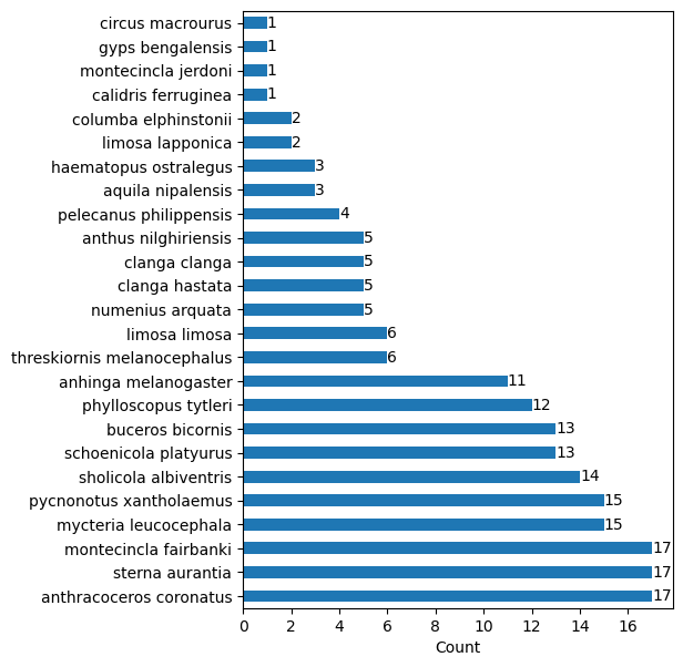
Fig.1 Bar plot of available species
The time domain plot explains the variation of signal amplitude with time and spectrogram reveals frequency variation with respect to time. The time domain plot and spectrogram are drawn to understand the pattern of the bird song/call.
The code snippet and the associated plot (Fig. 2 and Fig. 3) are as follows,
Time domain plot,
mple_df = audio_df.sample(n=1)
sample_species = sample_df['species'].iloc[0]
sample_sciname = sample_df['sci_name'].iloc[0]
sample_filename = sample_df['full_name'].iloc[0]
audio_data, Fs = librosa.load(audio_path+sample_filename)
data_stft = librosa.stft(audio_data)
dB = librosa.amplitude_to_db(abs(data_stft))
fig, ax = plt.subplots(figsize=(7, 3))
librosa.display.waveshow(audio_data,sr=Fs)
plt.title('Bird Call of {} species ({})'.format(sample_species, sample_sciname))
ipd.Audio(audio_data, rate=Fs)
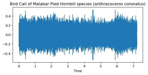
Fig. 2 Time domain plot of bird song/call
Spectrogram,
fig, ax = plt.subplots(figsize=(7, 3))
plt.title('Birdcall spectrogram of {} species ({})'.format(sample_species, sample_sciname))
librosa.display.specshow(dB, sr=Fs, x_axis='time', y_axis='hz')
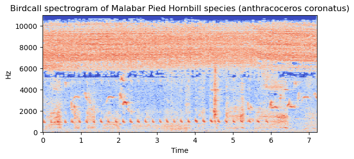
Fig.3 Spectrogram of audio signal in the sample data
For further understanding of the pattern in the audio signal, the audio duration all the samples are plotted as histogram, the code snippet and the figure (Fig. 4) drawn using the code are included in the following section,
durations = []
for index, row in tqdm(audio_df.iterrows(), total=audio_df.shape[0]):
file_name = row['full_name']
y, Fs = librosa.load(audio_path+file_name)
duration = librosa.get_duration(y=y, sr=Fs)
durations.append(duration)
fig, ax = plt.subplots(figsize=(6, 3))
plt.title('Histogram of Bird Call Durations')
plt.hist(durations, bins=20)
plt.xlabel('Time (seconds)')
plt.ylabel('Count')
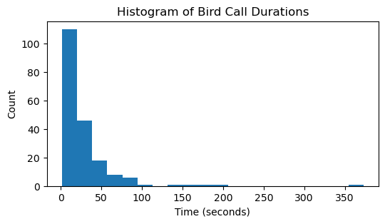
Fig. 4. Histogram of duration of Bird call
Using the data obtained from the spectrogram, a 2D tSNE plot was created. Even after multiple iterations, there was no clear clustering between the 25 classes of bird species.
The code snippet and the tSNE plot ( Fig.5) are as follows,
tsne = TSNE(n_components=2, perplexity=20.0, n_iter=2000,verbose=1)
z = tsne.fit_transform(spectro_df)
tsne_df = pd.DataFrame()
tsne_df["y"] = ylabels
tsne_df["component 1"] = z[:,0]
tsne_df["component 2"] = z[:,1]
sns.scatterplot(x="component 1", y="component 2", hue=tsne_df.y.tolist(),
palette=sns.color_palette("hls", 25),
data=tsne_df).set(title="Spectrogram T-SNE projection")

Fig.5 tSNE projection of spectrogram
The principal component analysis (PCA) of spectrogram is carried out. PCA reveals that the first 9 principal components are sufficient to capture the 95 % of variance in the spectrogram features.
The code snippet for PCA and the figure (Fig. 6) generated using the code are as follows,
pca_obj = PCA()
pca_obj.fit(spectro_df)
plt.plot(np.cumsum(pca_obj.explained_variance_ratio_))
plt.xlabel('Number of Components')
plt.ylabel('Cumulative Explained Variance');
print(np.cumsum(pca_obj.explained_variance_ratio_)[:10])
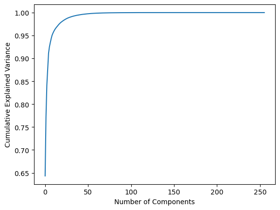
Fig.6 Cumulative explained variance of number of PCA components
Inferences from EDA
The key observations from the EDA can be summarised as follows,
1. There are 194 bird song/call recordings collected from https://xeno-canto.org/
2. The histogram of number of recoding’s per species shows a tailed distribution
3. The time domain and spectrogram plots are plotted. Spectrogram plots are having clear visual patterns and may perform well with CNN based models.
4. Most of the recordings are of nearly 2 minutes duration
5. The TSNE plot shows no clear separation between classes
6. The PCA analysis shows that first 9 principal components are enough to capture 95% of the variance in spectrogram features.
Modeling
Three types of deep learning models with same architecture are tried. The difference is in the features used for each model. Model 1 uses simple raw audio data as input. The second model uses Fast Fourier transformed (FFT) raw audio. The third model uses features extracted through feature engineering which combines Fourier transformed raw audio and Mel frequency Cepstral coefficients (MFCC) of raw audio.
The function for creating deep neural network (DNN) is given below,
def create_n_return_dnn():
dnn_model = Sequential()
dnn_model.add(Dense(128, kernel_initializer=RandomUniform(minval=-0.05,
maxval=0.05), kernel_regularizer=l2(0.001),
activation='relu'))
dnn_model.add(Dense(256, kernel_initializer=RandomUniform(minval=-0.05,
maxval=0.05), kernel_regularizer=l2(0.001),
activation='relu'))
dnn_model.add(Dropout(0.2))
dnn_model.add(Dense(512, kernel_initializer=RandomUniform(minval=-0.05,
maxval=0.05), kernel_regularizer=l2(0.001),
activation='relu'))
dnn_model.add(Dropout(0.2))
dnn_model.add(Dense(256, activation='relu', kernel_regularizer=l2(0.001)))
dnn_model.add(Dense(128, activation='relu', kernel_regularizer=l2(0.001)))
dnn_model.add(Dropout(0.2))
dnn_model.add(Dense(NCLASSES, activation='softmax', kernel_regularizer=l2(0.001)))
return dnn_model
The architecture and model summary is shown below,
Model: “sequential”
_________________________________________________________________
Layer (type) Output Shape Param #
=================================================================
dense (Dense) (None, 128) 5644928
dense_1 (Dense) (None, 256) 33024
dropout (Dropout) (None, 256) 0
dense_2 (Dense) (None, 512) 131584
dropout_1 (Dropout) (None, 512) 0
dense_3 (Dense) (None, 256) 131328
dense_4 (Dense) (None, 128) 32896
dropout_2 (Dropout) (None, 128) 0
dense_5 (Dense) (None, 25) 3225
=================================================================
Total params: 5,976,985
Trainable params: 5,976,985
Non-trainable params: 0
The code to generate FFT features is as follows,
X_train_fft = []
for train_row in tqdm(X_train_raw):
X_train_fft.append(np.abs(np.fft.fft(train_row)))
X_train_fft = np.vstack(X_train_fft)
X_test_fft = []
for test_row in tqdm(X_test_raw):
X_test_fft.append(np.abs(np.fft.fft(test_row)))
X_test_fft = np.vstack(X_test_fft)
The code to generate MFCC features is as follows,
X_train_MFCC = []
for train_row in tqdm(X_train_raw):
mfcc = librosa.feature.mfcc(y=train_row, sr=FS)
mfcc = np.sum(mfcc, axis=0)
X_train_MFCC.append(mfcc)
X_train_MFCC = np.vstack(X_train_MFCC)
X_test_MFCC = []
for test_row in tqdm(X_test_raw):
mfcc = librosa.feature.mfcc(y=test_row, sr=FS)
mfcc = np.sum(mfcc, axis=0)
X_test_MFCC.append(mfcc)
X_test_MFCC = np.vstack(X_test_MFCC)
The best model among all models trained was the FFT+MFCC , the accuracy and loss plot (Fig. 7) for both train and test data is shown below,
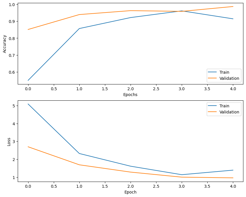
Fig. 7 Accuracy and loss plot of the third deep learning model (FFT+MFCC)
Results
The validation accuracy and F1 score (Table.1) which are opted as the performance metric for this case study are summarised for all the models in the table below,
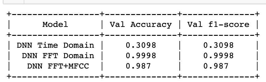
Table.1 Performance metric of all models using deep learning techniques
End note
The best performing model, which is FFT+MFCC is deployed as a streamlit application.
You can check the deployed model at https://roshnash-streamlit-r-main-uxj8lk.streamlit.app/
The deployed code is available at https://github.com/roshnash/streamlit_r
This article is first published online by myself at medium.
This article is documentation of project based on machine learning/deep learning technique. Similar documentations can be found in the following links,
1. https://intuitivetutorial.com/2023/04/14/perovskites/
2. https://intuitivetutorial.com/2022/11/16/primary-or-metastasis-classifier-using-deep-learning/
3. https://intuitivetutorial.com/2022/09/18/breast-cancer-survivability-classifier/