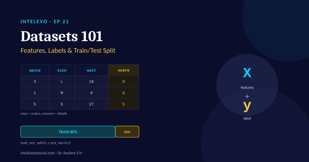
Every machine learning model starts with data. But before you train anything, you need to understand your dataset first. This article walks through three ideas that show up in almost every ML project: features, labels, and the train test split. It pairs with Episode 21 of the Intelevo YouTube series, so watch the video first if you prefer to learn by ear, then use this post to review the details at your own pace.
By the end, you’ll know exactly how to look at any dataset and answer three questions. What are the inputs? What’s the answer you’re predicting? And how do you test your model honestly, instead of fooling yourself? These three questions sound simple, yet they trip up more beginners than any algorithm ever does. So, let’s slow down and build the intuition properly, one small idea at a time.
Why This Topic Matters
Here’s the problem. Most beginners jump straight into fitting a model. They skip the step where they actually understand their data. As a result, they get confused later when their code throws shape errors, or worse, when their “accurate” model fails completely on new data.
So, before we touch scikit-learn’s fit function, we need a mental model for the dataset itself. That’s what this article covers. And to keep things simple, we’ll lean on one analogy throughout: a restaurant order pad.
This matters even more once you start comparing models, tuning hyperparameters, or reporting results to someone else. If your understanding of features, labels, and the train test split is shaky, every later step inherits that shakiness. Get this foundation right first, and everything downstream becomes noticeably easier.
The Order Pad Analogy
Picture a waiter taking orders at a busy restaurant. For every table, they jot down a few details: the spice level requested, the size of the order, and how long the table waited for their food. Then, at the end of the night, one more detail gets added: whether that table sent a compliment back to the chef.
That order pad is a dataset. Every detail the waiter wrote down before the meal is something they already knew. The compliment, on the other hand, only exists after the meal happens. That distinction — known beforehand versus revealed afterward — is the entire foundation of features and labels. Keep this picture in your mind. It’ll make every section below click faster.
What Exactly Is a Dataset?
In plain terms, a dataset is just a table. In Python, pandas calls this table a DataFrame. Each row represents one example, like one restaurant order. Each column represents one detail about that example, like spice level or wait time.
Here’s a simple example:
| spice_level | size | wait_time_min | satisfaction |
|---|---|---|---|
| 3 | Large | 18 | 9 |
| 1 | Medium | 9 | 8 |
| 5 | Small | 27 | 5 |
| 2 | Large | 12 | 9 |
Look closely, and you’ll notice the last column stands apart from the rest. That’s intentional. It represents the outcome, not an ingredient. We’ll come back to that in a moment.
First, though, notice how familiar this shape already is. If you’ve ever built a spreadsheet in Excel or Google Sheets, you’ve already worked with rows and columns like this. A dataset isn’t some exotic new structure. It’s a table you already understand, just with a new vocabulary attached to it.
Features: The Ingredients You Already Know
Now let’s zoom into the first three columns: spice level, size, and wait time. In machine learning, these are called features. A feature is any piece of information you already have before the outcome happens.
Think of it like a recipe card. You list your ingredients before the dish even exists. Similarly, features are the “ingredients” of your prediction — known in advance, ready to feed into a model.
In code, we collect these columns into a variable called X, always capitalized. Here’s how that looks:
X = data[["spice_level", "size", "wait_time"]]
print(X.head())
# Out: the ingredients, one row per order
That’s it. X now holds every column you’d know about an order the moment it comes in. Nothing here depends on the future. If you knew it before the dish came out, it’s a feature. Simple as that.
Labels: The Answer You’re Predicting
Next, let’s look at the satisfaction column. This is called the label, and in code, we always name it y, lowercase.
Think of it as the compliment slip. Nobody writes down a customer’s happiness before they’ve even tasted the food. That information only exists after the fact. Similarly, a label is the outcome your model is trying to predict, and it only becomes available once the event has already happened.
Here’s the code:
y = data["satisfaction"]
print(y.head())
# Out: the answer, revealed after the meal
Now compare this with the feature block above. Features are known upfront. Labels are revealed afterward. That’s the entire difference between X and y, and once it clicks, half of supervised machine learning starts to make sense.
Features vs Labels: A Quick Comparison
To make sure it sticks, here’s a side-by-side view.
Features (X)
- What it is: known before the outcome
- Analogy: the order pad details
- Code:
data.drop("satisfaction", axis=1)
Labels (y)
- What it is: the outcome itself, after the fact
- Analogy: the compliment slip
- Code:
data["satisfaction"]
Notice how short both code snippets are. That’s not an oversimplification. Splitting features from labels really is that straightforward, once your dataset is clean and organized.
Putting It Together: Loading Data and Splitting X and y
Let’s combine everything into one working example. First, import pandas. Then, load your CSV file. After that, split the data into X and y.
import pandas as pd

data = pd.read_csv("orders.csv")
X = data.drop("satisfaction", axis=1)
y = data["satisfaction"]

print(X.shape, y.shape)
# Out: (500, 3) (500,)
In this example, we have 500 orders, three ingredients each, and one compliment column pulled aside. Four lines of code, and your dataset is fully prepared for the next step.
Why We Hold Data Back Before Testing
Here’s a question worth pausing on. Once you have X and y, why not just train your model on all of it and call it done?
Think about a chef testing a brand-new dish. They never trust only the people who watched it get cooked. Those tasters already know too much about the recipe. Instead, a good chef brings in someone new, someone who has never seen the dish before, for an honest verdict.
Machine learning works exactly the same way. A model that only sees questions it already memorized isn’t proving anything useful. Being perfect on familiar data is easy. Being accurate on unseen data is what actually proves a model works. That’s why every serious ML workflow holds back a portion of data purely for testing.
Without this step, you risk a problem called overfitting. In simple terms, overfitting happens when a model memorizes the training data instead of learning the underlying pattern. It performs beautifully on familiar examples, then falls apart the moment it meets something new. A proper train test split catches this problem early, before it costs you time, money, or credibility in front of a client.
The Train-Test Split, Explained
This is where the train test split comes in. Instead of feeding a model 100% of your data, you divide it into two separate groups.
- Training set: typically 80% of your data. The model learns patterns from this portion.
- Test set: typically 20% of your data. The model never sees this portion during training. You use it only to judge performance honestly afterward.
Here’s the code, using scikit-learn:
from sklearn.model_selection import train_test_split

X_train, X_test, y_train, y_test = train_test_split(
    X, y, test_size=0.2, random_state=42)

print(X_train.shape, X_test.shape)
# Out: 400 orders to learn from, 100 to judge honestly
Notice the test_size=0.2 parameter. That single number controls the split ratio. It simply means one in every five orders gets set aside for testing. Nothing more complicated than that.
A Quick Gut-Check
Let’s test your understanding with a quick scenario. Suppose you train a model on all 500 orders, and it predicts every single one correctly. Does that prove the model works on new customers?
Take a moment to think it over.
The answer is no. That model has only proven itself on data it already memorized. Grading yourself on questions you already know the answers to isn’t a real test. It’s just a memory check. This is exactly why the train test split matters so much in practice.
You’ve Actually Used This Idea Before
Here’s some good news: you already understand this concept, even if you’ve never coded it. Consider these everyday examples.
First, exam preparation. You study practice questions, then get graded on questions you’ve genuinely never seen before.
Second, a recipe taste test. A chef tests a new dish on a stranger, not just on the kitchen staff who cooked it.
Third, a movie test screening. Studios show a rough cut to a fresh audience before the official release, specifically to get honest, unbiased feedback.
Fourth, quality control in factories. Workers pull random items off the production line to inspect, rather than testing only the ones they’ve already double-checked.
In every case, holding something back to judge honestly is a habit you already trust. Machine learning simply gives that habit a formal name: the train test split.
Pro Tips and Common Pitfalls
Before wrapping up, here are four practical habits that will save you real headaches later.
First, always set random_state. This locks in the same split every time you run your code. Without it, your results shuffle unpredictably each time you rerun the script, making debugging much harder.
Second, shuffle your data before splitting. If your file happens to have all of Monday’s orders sitting at the top, an unshuffled split could hand you a test set made entirely of Mondays. That’s a biased, misleading evaluation.
Third, use stratify for imbalanced labels. Suppose only one in twenty orders results in a complaint. Setting stratify=y ensures that same ratio appears in both your training and test sets, so your evaluation stays representative.
Fourth, and most importantly, never let test data influence training. Peeking at test results while tuning your model is like grading your own exam before turning it in. Once that happens, the score means nothing anymore. Keep that boundary strict, no exceptions.
Putting It All Together: A Full Code Walkthrough
Here’s the complete workflow, start to finish, combining everything covered above.
import pandas as pd
from sklearn.model_selection import train_test_split

data = pd.read_csv("orders.csv")
X = data.drop("satisfaction", axis=1)
y = data["satisfaction"]

X_train, X_test, y_train, y_test = train_test_split(
    X, y, test_size=0.2, random_state=42)

print("Train:", X_train.shape, "Test:", X_test.shape)
# Out: Train: (400, 3) Test: (100, 3)
One file goes in. Four pieces come out. X_train and y_train teach the model. X_test and y_test judge it honestly afterward. This single cell is worth running before training any model in your project, every single time.
Key Takeaways
Let’s recap everything in a few short points.
- A dataset is simply a table. Rows represent examples, and columns represent details.
- Features (
X) are everything known before the outcome happens. - Labels (
y) are the outcome itself, revealed only afterward. - The train test split divides your data so evaluation stays honest and unbiased.
- Settings like
random_state, shuffling, andstratifykeep your split fair and reproducible.
Once these five ideas feel natural, you’re genuinely ready to prepare data for any machine learning model, not just the toy examples in a tutorial.
Common Questions About the Train Test Split
What is a good train test split ratio? An 80/20 split works well for most small to medium datasets. For very large datasets, a 90/10 split is often enough, since even 10% still represents a huge number of examples.
Can I skip the train test split if my dataset is small? No, and this is exactly when it matters most. Small datasets are more prone to overfitting, so a proper train test split becomes even more important, not less.
Does the train test split guarantee my model is accurate? Not by itself. It only guarantees an honest evaluation. Accuracy still depends on your features, your model choice, and how well your data represents the real-world problem.
Should I always use random_state=42? The number itself doesn’t matter. What matters is picking any fixed number and sticking with it, so your split stays reproducible every time you rerun your code.
What’s Next
Real datasets rarely arrive perfectly clean. Sometimes a spice level goes unmarked. Sometimes a wait time never gets logged. In the next episode, Episode 22, we tackle exactly that problem: data cleaning, with a specific focus on handling missing values. If today’s post made sense, that next one will feel like a natural continuation.
Watch the Full Video
This article accompanies Episode 21 of the Intelevo YouTube series, where every example here gets explained live, with visuals and a walkthrough of the code in action. If you’d rather watch it unfold step by step, head over to the Intelevo channel and check out the full episode. And if this post helped clarify things, consider leaving a comment on the video to let us know what clicked for you.