Data preprocessing breaks more machine learning projects than bad models do. You impute missing values. You scale numbers. You encode categories. Then you repeat all of it, by hand, on your test set. One typo creeps in, and your results quietly fall apart. This is exactly why ML pipelines in scikit-learn exist, and this article walks you through them, step by step.
This post is the companion piece to Episode 60 of the Intelevo Machine Learning series on YouTube. Watch the full video for a visual, code-along walkthrough, or use this article as your quick-reference guide. Either way, by the end, you’ll understand Pipeline and ColumnTransformer well enough to use them confidently in your own projects.
Why Manual Preprocessing Breaks Projects
Let’s start with the pain point. Most beginners preprocess data like this: they impute missing values, scale the numeric columns, encode the categorical ones, and only then train a model. It works, at first. But problems show up quickly.
First, you end up copy-pasting code. You write the same imputer and scaler logic once for your training set and once for your test set. Over time, the two versions drift apart, and nobody notices until the model behaves strangely in production.
Second, silent data leakage creeps in. If you fit a scaler on your entire dataset before splitting it into train and test, that scaler already “knows” something about your test set. Your validation score looks fantastic. Unfortunately, it’s lying to you.
Third, deployment becomes fragile. You hand your trained model to a colleague or push it to production, but you forget one preprocessing step. The model breaks, often without a clear error message. Debugging this in production is nobody’s idea of fun.
So, how do you avoid all three problems at once? You bundle every step into one object. That’s exactly what a pipeline does.
The Big Idea: Think of a Factory Assembly Line
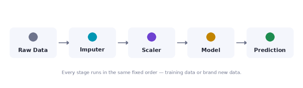
Here’s a simple way to picture a pipeline. Imagine a factory assembly line. Raw material enters at one end. It passes through fixed stations, in a strict order: cut, weld, paint. A finished, identical product exits the other end, every single time.
A Pipeline is that assembly line, but for data. Every station runs in exactly the same order, whether you feed it training data today or a brand-new row next year. Nothing gets skipped. Nothing gets reordered by accident.
Keep this image in mind. It will make every other concept in this article click into place.
Meet the First Tool: sklearn.pipeline.Pipeline
Pipeline, from sklearn.pipeline, chains your preprocessing steps and your model into a single object. As a result, you call .fit() once and .predict() once, and every station runs automatically in between.
Here’s the simplest possible pipeline, using our numeric-only example:
from sklearn.pipeline import Pipeline
from sklearn.impute import SimpleImputer
from sklearn.preprocessing import StandardScaler

numeric_pipe = Pipeline([
    ("impute", SimpleImputer(strategy="median")),
    ("scale", StandardScaler()),
])
Notice the structure. Each step is a tuple: a name, followed by a transformer. SimpleImputer fills missing values with the column median. StandardScaler then rescales the result. Because both steps live inside one Pipeline object, calling numeric_pipe.fit_transform(X) runs them in order, automatically.
This is the habit worth building today: everything after your raw data lives inside the pipeline. You never touch intermediate steps by hand again.
Why This Actually Prevents Data Leakage
Let’s get specific about why this matters so much, because it’s easy to underestimate.
Without a pipeline, imagine you scale your data first, across the entire dataset, and only split into train and test afterward. Your scaler has already seen the test set’s mean and standard deviation. It learned something it shouldn’t know yet. Your validation score looks great, but only because the model quietly peeked at information it will never have in the real world.
With a pipeline, the fix is automatic. When you call .fit() on training data only, every station inside the pipeline — the imputer, the scaler, everything — learns its parameters strictly from that training data. When you then call .transform() or .predict() on test data, the pipeline reuses those same learned parameters. It never refits on the test set. As a result, your test set stays genuinely unseen, and the score you get back means something real.
This single habit is often the difference between a model that performs well in a notebook and one that performs well in production.
The Catch: Real Data Isn’t All One Ingredient
So far, so good. But here’s a wrinkle. A single assembly line assumes every item passing through it has the same shape. Real-world tables rarely cooperate.
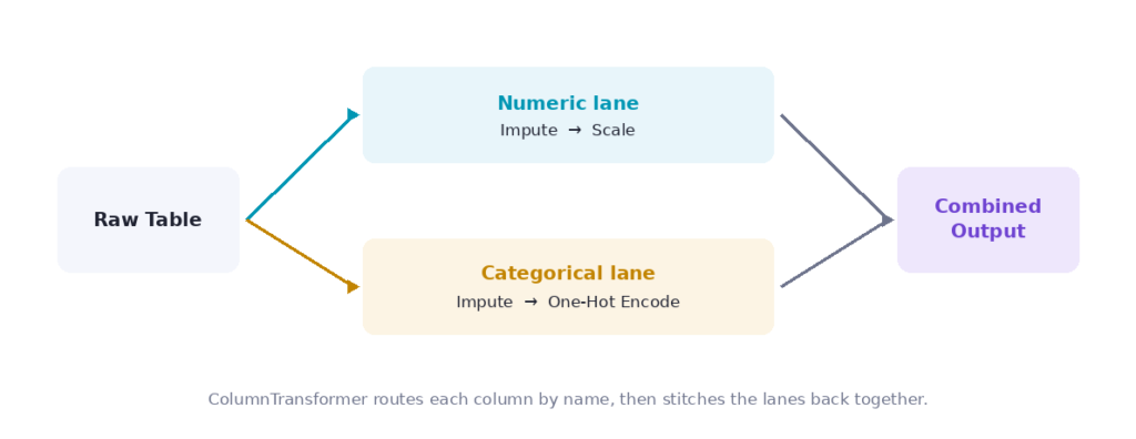
Consider a customer dataset with four columns: age, income, city, and gender. The first two are numeric. The last two are categorical. Numeric columns need imputing and scaling. Categorical columns need imputing and encoding — a completely different transformation.
One conveyor belt can’t run two different processes on two different lanes at once. Trying to force StandardScaler onto a text column like city will simply throw an error. Clearly, you need a router: something that sends each column down the correct lane, based on its type.
Meet the Second Tool: sklearn.compose.ColumnTransformer
That router is ColumnTransformer, from sklearn.compose. It splits your table by column, sends each group down its own mini pipeline, and then stitches the results back together, side by side.
Here’s how you build both lanes:
from sklearn.compose import ColumnTransformer
from sklearn.preprocessing import OneHotEncoder

numeric_cols = ["age", "income"]
categorical_cols = ["city", "gender"]

numeric_pipe = Pipeline([
    ("impute", SimpleImputer(strategy="median")),
    ("scale", StandardScaler()),
])

categorical_pipe = Pipeline([
    ("impute", SimpleImputer(strategy="most_frequent")),
    ("encode", OneHotEncoder(handle_unknown="ignore")),
])

preprocess = ColumnTransformer([
    ("num", numeric_pipe, numeric_cols),
    ("cat", categorical_pipe, categorical_cols),
])
Notice the pattern again. Each entry in ColumnTransformer is a tuple: a name, a transformer (in this case, an entire mini pipeline), and the list of column names it applies to. The categorical lane imputes missing values using the most frequent category, then applies OneHotEncoder. The handle_unknown="ignore" argument matters here too — it stops the pipeline from crashing if a brand-new category shows up later, after deployment.
Each column is told exactly which lane to take, by name. The router never mixes them up, and you never have to manually slice your DataFrame again.
Putting Both Tools Together
Now for the payoff. You wrap the entire ColumnTransformer inside one more outer Pipeline, alongside your model. The result is a single object that takes raw data in and produces predictions out, with every transformation handled automatically in between.
from sklearn.linear_model import LogisticRegression
from sklearn.model_selection import cross_val_score

model = Pipeline([
    ("prep", preprocess),
    ("clf", LogisticRegression()),
])

model.fit(X_train, y_train)          # one call trains everything
model.predict(X_test)                # one call scores everything

scores = cross_val_score(model, X, y, cv=5)
Look closely at how little code this takes. model.fit(X_train, y_train) trains the imputers, the scaler, the encoder, and the classifier, all in one call, all in the correct order. model.predict(X_test) applies every one of those fitted transformations before generating a final prediction.
Even better, you can hand the entire model object straight to cross_val_score. Scikit-learn automatically re-fits the whole pipeline, fresh, on every fold. You get a clean, leak-proof cross-validation score, without writing a single extra line of preprocessing code.
Four Concrete Wins From This One Habit
Let’s tie the benefits together, because they compound quickly once you adopt this pattern.
Leak-proof by design. Because fitting happens only on training folds, every score you report — cross-validation or otherwise — genuinely reflects how your model will perform on new data.
Far less code. You never duplicate imputer or scaler logic for train and test separately. You write the transformation logic exactly once.
Full reusability. The same fitted pipeline transforms and predicts on any new batch of data, whether that’s next month’s customers or a completely different dataset with the same schema.
Deployment-ready. You can save the entire pipeline with a single joblib.dump() call. Your preprocessing logic travels with your model, wherever you deploy it. Nobody on your team needs to remember which scaler you used, or in what order.
import joblib

joblib.dump(model, "pipeline_model.pkl")

# later, in a completely different script or service
loaded_model = joblib.load("pipeline_model.pkl")
loaded_model.predict(new_data)
That’s the entire deployment story. You don’t ship a model file plus a separate preprocessing script plus a page of instructions. You ship one file. It works everywhere, exactly the way it worked in your notebook.
Common Pitfalls to Avoid
A few mistakes trip up even experienced practitioners, so it’s worth naming them directly.
Fitting outside the pipeline. If you call scaler.fit() on your full dataset before building the pipeline, you’ve already defeated the purpose. Keep every fit call inside the pipeline, and only ever call it on training data.
Forgetting the remainder parameter. By default, ColumnTransformer silently drops any column you didn’t explicitly list. If you need to keep an untouched column, set remainder="passthrough".
Column name typos. A misspelled column name can fail silently in some setups, so always double-check that your column lists match your DataFrame exactly.
Cross-validating after fitting. Always pass the unfit pipeline into cross_val_score. It re-fits the pipeline, fresh, on every single fold automatically. If you fit it first and then cross-validate, you reintroduce the leakage you were trying to avoid.
Avoid these four traps, and your pipelines will behave exactly as expected, every time.
Recap: It’s Just an Assembly Line for Data
Let’s bring everything back to the core idea. A Pipeline chains steps in a fixed order, so one .fit() call and one .predict() call handle everything, and nothing ever gets forgotten. A ColumnTransformer routes numeric and categorical columns to their own mini pipelines, then recombines the results. Together, they fit only on training data, so every score you compute stays genuinely trustworthy. And because the entire thing behaves as a single object, it’s reusable, testable, and ready for deployment exactly as it is.
Once you build a few of these, writing preprocessing code by hand will start to feel unnecessary. That’s the goal.
Quick FAQ
Do I need ColumnTransformer if my data is all numeric? No. If every column is numeric, a plain Pipeline with an imputer and a scaler handles everything. Reach for ColumnTransformer only when you mix data types, such as numbers alongside categories or text.
Can I add more than two lanes? Yes. ColumnTransformer accepts as many entries as you need. For instance, you might add a third lane for text columns, using TfidfVectorizer instead of OneHotEncoder. The pattern stays identical: name, transformer, column list.
Does a pipeline slow down training? Barely, if at all. Each station still runs the same underlying scikit-learn code. You gain organization and safety, and you lose essentially nothing in speed.
Why does this matter for building ML pipelines in scikit-learn specifically? Because scikit-learn’s Pipeline and ColumnTransformer integrate directly with GridSearchCV, cross_val_score, and model persistence tools. You get leak-proof preprocessing and full compatibility with the rest of the ecosystem, in one step.
What’s Next: Introduction to Ensemble Learning
In Episode 61, we move on to ensemble learning: why combining many simple models genuinely beats relying on just one. We’ll cover bagging, boosting, and voting, and how each technique blends multiple models into a single, stronger predictor. Fittingly, every model in that episode gets trained inside a pipeline, exactly like the ones you just built here.
Watch the Full Video
This article covers the core ideas, but the video walks through every diagram, every code cell, and every explanation out loud, at a pace that’s easy to follow. If you found this guide useful, head over to the Intelevo YouTube channel and watch Episode 60 in full. While you’re there, please like the video, subscribe for future episodes, and leave your questions in the comments ,every comment genuinely shapes what gets covered next.
Mastering ML pipelines in scikit-learn pays off on nearly every project you touch afterward. Once you see raw data flow cleanly through imputers, scalers, encoders, and a model, all inside one object, you won’t want to preprocess any other way.