Every machine learning course starts the same way. Someone hands you a clean CSV file. The columns already make sense. The categories are already encoded. The scaling is already done. You load it, you split it, you train a model, and it works.
Then you try this on your own data, and none of that is true.
Real data arrives messy. Dates sit there as plain text. Categories need converting into numbers. Some columns matter enormously, and others are just noise pretending to be useful. Before any model can do its job, someone has to decide what the model actually gets to see. That decision has a name: feature engineering and feature selection. And it is arguably the single most underrated skill in applied machine learning.
This post walks through both halves of that skill in plain language, with a real dataset and runnable Python code. By the end, you will know exactly how to turn raw, unprocessed columns into model-ready features, and how to decide which of those features are actually worth keeping.
This article is associated with episode 79 of Intelevo ML tutorial series
Why Feature Engineering and Feature Selection Matter More Than the Algorithm
Here’s an analogy worth keeping in mind for this entire post: raw data is a pantry, not a meal. A pile of ingredients does not feed anyone until someone measures, chops, and combines them into something edible. Raw data works the same way. A model cannot “cook” with a raw date column or an unencoded category. It needs prepared inputs.
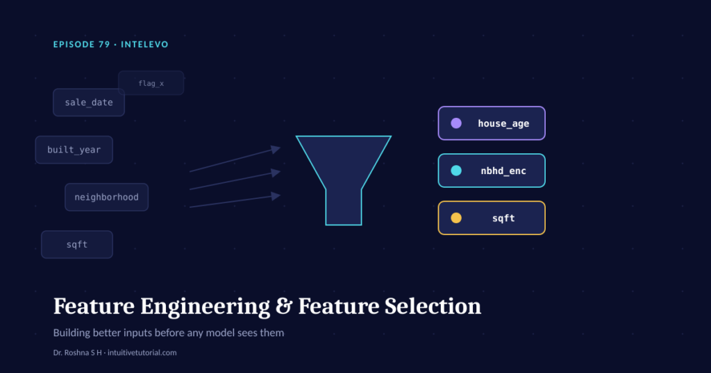
Feature engineering and feature selection split that prep work into two halves. Feature engineering adds. It builds new columns, transforms existing ones, and combines raw fields into signals a model can actually use. Feature selection removes. It looks at every feature — old and new — and decides which ones earn a place in the final model, and which ones are just adding noise.
Put those two ideas together in one sentence, and you get the entire premise of this post: feature engineering turns raw columns into useful signals, and feature selection decides which of those signals are actually worth keeping.
It’s tempting to think the fix for a mediocre model is a fancier algorithm. Often, it isn’t. A well-engineered feature can outperform switching from linear regression to a gradient-boosted ensemble. Better inputs consistently beat bigger models, and that single fact is why feature work deserves as much attention as model selection.
Meet the Dataset
To keep things concrete, imagine a table of house sales. Each row is one house, with six raw columns:
| House ID | Sqft | Built Year | Neighborhood | Sale Date | Price |
|---|---|---|---|---|---|
| 1 | 1,340 | 1998 | Riverside | 2023-05-14 | $285,000 |
| 2 | 2,105 | 2015 | Lakeview | 2023-06-02 | $412,500 |
| 3 | 980 | 1975 | Oldtown | 2023-03-21 | $189,900 |
| 4 | 1,760 | 2008 | Riverside | 2023-07-09 | $334,000 |
Nothing here is model-ready yet. Built Year and Sale Date, in particular, aren’t useful on their own. But look at the gap between them. The difference between the sale year and the built year gives you the house’s age at the time it sold — a number that means something to a buyer, and to a model. That gap is a feature waiting to be built, and it’s exactly where the engineering half of this post begins.
Feature Engineering: Turning Raw Columns Into Useful Signals
Feature engineering follows a consistent pattern: look at a raw column, decide what a model actually needs from it, and build that directly.
Step 1: Turn a Date Into Something Usable
A raw date, stored as text, tells a model nothing. The fix starts with converting it into an actual datetime object, which then lets you pull out anything useful hiding inside it.
import pandas as pd

df = pd.read_csv("houses.csv")
df["Sale_Date"] = pd.to_datetime(df["Sale_Date"])

# new feature: age at time of sale
df["House_Age"] = (df["Sale_Date"].dt.year
                    - df["Built_Year"])
df["Sale_Month"] = df["Sale_Date"].dt.month
pd.to_datetime() makes the year and month extractable in the first place. From there, House_Age is a genuinely new feature — one subtraction turns two nearly-useless columns into a single signal that correlates strongly with price. Sale_Month captures something different: seasonality. Homes may sell differently in June than they do in December, and that pattern is invisible until you extract it.
This is the core move of feature engineering. You’re rarely inventing information from nothing. You’re surfacing information that was already present in the raw data, just in a shape the model couldn’t use.
Step 2: Turn Categories Into Numbers
Neighborhood is text, and most models only understand numbers. Before it’s usable, it needs encoding.
df = pd.get_dummies(
    df,
    columns=["Neighborhood"],
    drop_first=True)

print(df.filter(like="Neighborhood_").columns)
get_dummies() creates one new column per neighborhood, each holding a 0 or a 1. This is called one-hot encoding, and it’s the standard way to hand categorical data to most machine learning algorithms. Notice the drop_first=True argument. It removes one of the generated columns on purpose — once a model knows a house isn’t in any of the other neighborhoods, it already knows which one is left. Keeping that final column would just be redundant, and redundant features cause their own problems later.
At this point, the dataset has grown. What started as six raw columns is now a wider table with House_Age, Sale_Month, and several neighborhood indicator columns added on. This is normal. Feature engineering almost always increases the column count before feature selection brings it back down.
Feature Selection: Deciding What’s Actually Worth Keeping
Once you’ve engineered a batch of new features, the next question is unavoidable: which of these actually help? This is where feature selection takes over, and it generally happens through three families of methods.
Filter Methods
Filter methods score every feature on its own, before any model exists. They’re fast, and they’re a reasonable first pass for removing obvious noise.
from sklearn.feature_selection import \
    VarianceThreshold

corr = df.corr(numeric_only=True)["Price"]
weak = corr[corr.abs() < 0.05].index

selector = VarianceThreshold(threshold=0.01)
selector.fit(df[numeric_cols])
df.corr() shows how strongly each numeric column moves together with Price. A value near zero means that column barely predicts anything on its own, and weak collects those columns as the first drop candidates.
Correlation alone doesn’t catch everything, though. VarianceThreshold catches a second, sneakier failure: a column that barely varies at all, like a flag that’s almost always the same value across every row. A feature like that can’t help a model separate anything, no matter what its correlation with the target happens to be.
The tradeoff with filter methods is that they look at each feature in isolation. They can miss a feature that only becomes useful in combination with another one.
Wrapper Methods
Wrapper methods take a slower, more thorough approach. Instead of scoring features individually, they try different subsets of features on an actual model and keep whichever combination performs best — commonly through an approach called recursive feature elimination. Because this means training many models rather than one, wrapper methods cost more time and compute, but they can catch interactions that filter methods miss entirely.
Embedded Methods
Embedded methods sit in between. Selection happens as a side effect of training a model, rather than as a separate calculation beforehand.
from sklearn.ensemble import \
    RandomForestRegressor

rf = RandomForestRegressor(random_state=42)
rf.fit(X_train, y_train)

importances = pd.Series(
    rf.feature_importances_, index=X_train.columns
).sort_values(ascending=False)

print(importances.head(5))
A trained Random Forest already knows which columns it leaned on most heavily to predict price. feature_importances_ scores every column directly — higher means the model used it more during training. Because this ranking comes for free once the model is fit, embedded methods are one of the most practical starting points for feature selection on real projects.
In practice, these three approaches aren’t mutually exclusive. A common, sensible order is to filter first to cut the obvious noise, and then let a wrapper or embedded method handle the more nuanced decisions among what’s left.
More Feature Engineering Techniques Worth Knowing
The date-splitting and encoding examples above cover two of the most common situations you’ll run into, but feature engineering and feature selection cover a wider toolkit than just those two moves. A few other techniques come up often enough that they’re worth knowing before you hit them in your own data.
Scaling. Many algorithms, including K-Means and gradient descent-based models, measure distance directly. If one column is in the thousands and another sits between zero and one, the larger column silently dominates every calculation. StandardScaler rewrites every column onto the same footing, using the formula z = (x − mean) / std, so no single column overwhelms the others just because of its raw magnitude.
Log transforms. Price, income, and population data are almost always skewed — a small number of very large values stretch the distribution out. Taking the logarithm of a skewed column compresses those extreme values and often makes patterns easier for a model to learn. It’s a one-line transform with a disproportionate payoff on financial and demographic data.
Binning. Sometimes a continuous variable is more useful as a category. Turning House_Age into buckets like “new,” “established,” and “older” can help simpler models capture non-linear relationships that a single continuous number would otherwise hide from them.
Interaction features. Two columns that aren’t individually predictive can become powerful when combined. Square footage divided by number of bedrooms, for instance, often reveals something neither column tells you alone. This is also exactly the kind of relationship that filter-based selection methods tend to miss, since they only look at one column at a time — another good reason not to rely on filtering alone.
None of these techniques are exotic. They’re small, deliberate transformations, applied one at a time, based on what a particular column actually needs. That’s the entire craft of feature engineering: noticing what a raw column is missing, and building the specific thing that fixes it.
Why This Matters Beyond a Single Model
Good feature engineering and feature selection pay off in three concrete ways.
Higher accuracy. A well-engineered feature can outperform switching to a fancier algorithm. Sometimes the honest fix for a mediocre model isn’t a better architecture — it’s a better column.
Faster training. Fewer, more relevant features mean less noise for a model to sift through, which translates directly into shorter training times and lighter compute costs.
Easier to explain. A model built on eight meaningful, well-named features is far easier to justify to a stakeholder, a regulator, or a teammate than one built on eighty unexplained ones. Interpretability isn’t just a nice-to-have; it’s often a requirement.
Every model built after this stage inherits whatever decisions were made here. That’s exactly why feature engineering and feature selection deserve real attention rather than being treated as a quick preprocessing afterthought.
Three Mistakes That Quietly Ruin a Good Pipeline
A feature pipeline can run successfully and still be wrong. Watch for these three silent failure points.
Data leakage. This happens when a feature is built using information that wouldn’t actually be available at prediction time — for example, deriving a new feature from the final sale price itself. Leakage inflates your validation score dramatically, and then the model fails quietly once it’s deployed on real, unseen data.
Selecting before splitting. If you choose features using your entire dataset, including the portion you meant to hold out for testing, information from that test set leaks into your selection decision. Always perform feature selection using training data only.
Dropping too aggressively. Cutting features based on correlation with the target alone can miss a feature that only becomes meaningful when combined with another one. A cautious, staged approach to removing features avoids throwing away something useful too early.
What You’ll Remember Tomorrow
Strip away the code, and feature engineering and feature selection reduce to two questions, asked over and over on every project: what can I build, and what can I remove?
Engineer first. Dates, ratios, and encoded categories often do more for model performance than reaching for a more complex algorithm. Select second. Filter out the obvious noise, then let a wrapper or embedded method rank whatever’s left. Always select using training data only, and never let test data leak into that decision. And above all, remember that a feature only earns its place if it actually improves real validation performance — not because it seemed like a good idea at the time.
Frequently Asked Questions
What is the difference between feature engineering and feature selection? Feature engineering creates new columns from raw data — through transforms, encodings, or combinations of existing fields. Feature selection then decides which of those columns, old and new, actually earn a place in the final model. Engineering adds; selection removes. Most real projects need both, usually in that order.
Do I need feature selection if I’m using a Random Forest? Often less than you’d think, since tree-based models handle irrelevant features more gracefully than linear models do. But feature selection still helps — fewer features mean faster training, easier interpretation, and less risk of a model that appears to work but is quietly leaning on noise.
Should I always scale my data before feature selection? It depends on the method. Correlation-based filtering doesn’t require scaled data, but many wrapper and embedded methods, particularly anything relying on distance or regularization, do. When in doubt, scale after splitting into train and test sets, never before.
How many features are too many? There’s no fixed number — it depends on your dataset size and your model. A useful signal, though: if adding more features stops improving validation performance, or starts hurting it, you’ve likely crossed from “helpful signal” into “noise the model has to fight through.”
What’s Next
Today’s feature selection kept or dropped columns whole. Each one either stayed exactly as it was, or it left the dataset entirely. The next episode in this series takes a bolder approach: Principal Component Analysis, or PCA, compresses dozens of features into a small handful of brand-new ones that still capture almost all the original signal.
If you’ve ever ended up with too many good features and struggled to decide which ones to cut, PCA offers a different answer. Instead of choosing, you compress — keeping essentially everything, just reshaped into fewer dimensions. That’s where this series goes next.