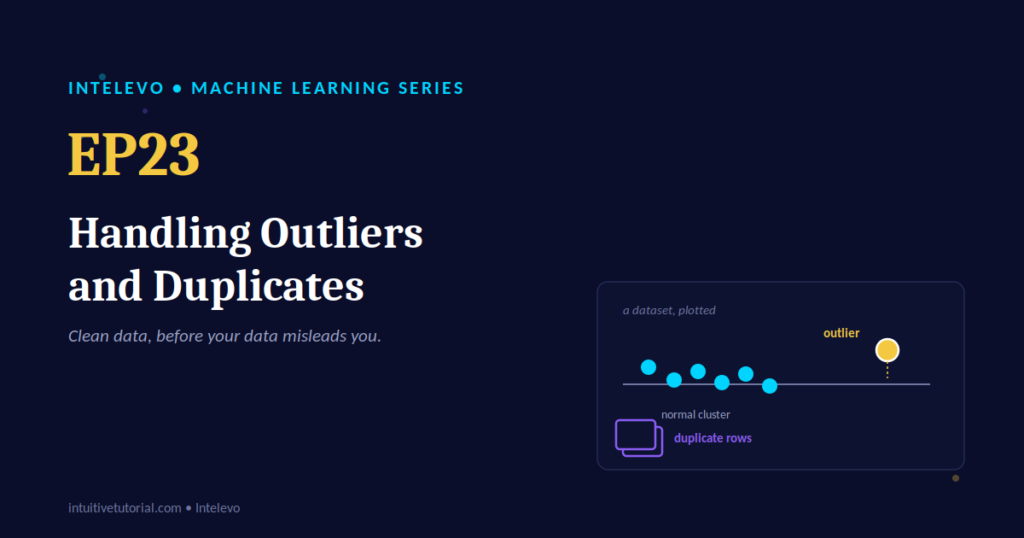
Every dataset lies to you a little. Not on purpose, but through two quiet troublemakers: outliers and duplicates. They hide in plain sight and skew your averages. They confuse your models. And most beginners never learn to catch them until something breaks.
This article is the companion piece to Episode 23 of the Intelevo machine learning series. We’ll walk through handling outliers and duplicates step by step, with runnable pandas code and almost no math. By the end, you’ll spot both problems in seconds, and you’ll know exactly what to do about them.
Let’s start with a picture.
The Bakery Conveyor Belt
Picture a bakery. Cookies roll off a conveyor belt toward the packing station. Most days, everything runs smoothly. But two small accidents can quietly wreck the batch report.
First, a giant, burnt cookie slips onto the scale by mistake. Suddenly, the “average cookie weight” for the entire batch looks way too high. Every other cookie is perfectly normal, yet one strange value throws off the whole picture. That’s an outlier — a value that simply doesn’t belong with the rest.
Second, the barcode scanner glitches. It logs one cookie into inventory twice. Now the “total cookies packed” count is wrong, even though nothing extra actually got baked. That’s a duplicate — the same information, counted more than once.
Keep this bakery picture in your mind. Every example in this article maps back to it.
Why This Matters Before You Train Any Model
Here’s the uncomfortable truth: a machine learning model can’t tell the difference between real signal and messy data. It just learns from whatever you feed it. So, if your dataset contains an outlier or a pile of duplicates, your model learns the wrong lesson.
Consider a simple example. You’re building a model to predict house prices. One row, due to a typo, lists a price of ₹5 crore instead of ₹50 lakh. Your model now thinks that kind of price is normal in that neighborhood. As a result, every prediction near that area skews upward.
Now add duplicates. Suppose the same listing accidentally appears five times in your training data. Your model starts treating that one house’s characteristics as five times more important than they should be. Consequently, the model overfits to that single example.
Clearly, cleaning your data before training isn’t optional. It’s the foundation everything else stands on.
What Exactly Is an Outlier?
An outlier is a data point that sits far outside where the rest of your data lives. It’s not necessarily wrong on purpose. Sometimes it’s a genuine data-entry mistake. Other times, it’s simply unusual.
Take this list of cookie weights, measured in grams:
weights = [42, 45, 41, 44, 43, 260, 46]
Six of these numbers cluster tightly around 44 grams. However, one value — 260 — stands wildly apart. If you plot these numbers on a number line, you’ll see it immediately: a tight cluster on one side, and one lonely point far away on the other. That lonely point is your outlier.
Outliers show up everywhere. A sensor might misfire and record a temperature of 999 degrees. A customer might accidentally type an extra zero into a price field. A rare, genuine event — like a once-in-a-decade stock spike — might also appear as an outlier, even though it’s completely real.
This is why detecting an outlier is only step one. Deciding what it means comes next.
Finding Outliers With the IQR Rule
You don’t need to eyeball every column to catch an outlier. One simple rule of thumb does most of the work: the IQR rule, short for interquartile range.
Here’s how it works. First, split your data into four equal parts, called quartiles. Q1 marks the value at the 25th percentile. Q3 marks the value at the 75th percentile. The interquartile range, or IQR, is the distance between them.
IQR = Q3 - Q1
lower = Q1 - 1.5 * IQR
upper = Q3 + 1.5 * IQR
That’s genuinely the only formula you need. Once you calculate the lower and upper bounds, anything below “lower” or above “upper” gets flagged as an outlier.
Visually, this maps perfectly onto a boxplot. The box in the middle represents your IQR — the range between Q1 and Q3. The lines extending outward are called whiskers. Any point that falls beyond those whiskers stands out immediately, just by looking at the chart. In fact, this is exactly why boxplots are such a popular first step in exploratory data analysis: they turn a math rule into a picture you can scan in seconds.
Notice something important here: this rule doesn’t need the mean or the standard deviation. Consequently, it stays reliable even when a few extreme values are already present, which is often the case in real datasets.
Code Demo: Spotting Outliers in Pandas
Let’s turn that formula into working code. Suppose you have a dataframe called df with a price column.
Q1 = df['price'].quantile(0.25)
Q3 = df['price'].quantile(0.75)
IQR = Q3 - Q1

lower = Q1 - 1.5 * IQR
upper = Q3 + 1.5 * IQR

outliers = df[(df['price'] < lower) | (df['price'] > upper)]
print(f"Found {len(outliers)} outlier rows")
Four lines. No loops. No manual scanning row by row. Pandas compares the entire column at once, and hands back every flagged row in a single dataframe called outliers. From there, you can inspect them, decide what to do, and move forward with confidence.
Found One. Now What?
Detecting an outlier is only half the job. The other half is deciding what to do with it. There’s no single right answer here — the correct choice depends on whether the value is a mistake or a genuine, rare event.
Remove it. If the value is clearly a data-entry error, like an extra zero typed by accident, dropping the row is often the simplest fix.
Cap it. This technique, sometimes called winsorizing, clips the value down to the nearest normal boundary instead of deleting the row entirely. You keep the row, but you tame the extreme value.
Keep it. If the outlier is rare but real — say, a genuine luxury purchase — removing it would throw away useful information. In cases like fraud detection, the outlier itself is often the whole point.
Capping, in code, takes just one line:
df['price'] = df['price'].clip(lower=lower, upper=upper)
This single line replaces every value below “lower” with “lower,” and every value above “upper” with “upper.” The rest of the column stays untouched.
What Exactly Is a Duplicate?
Now let’s shift to the second half of today’s topic: duplicates. A duplicate is simply a row that appears more than once. Sometimes the entire row is identical. Other times, just the important columns repeat — like the same customer ID showing up twice.
Consider this small order table:
| Order ID | Customer | Item | Amount |
|---|---|---|---|
| 1001 | Anu | Notebook | ₹120 |
| 1002 | Rahul | Pen Set | ₹80 |
| 1002 | Rahul | Pen Set | ₹80 |
| 1003 | Divya | Backpack | ₹950 |
Notice order 1002. It appears twice, back to back, completely identical. That second row isn’t a new order. It’s the same order, counted again. If you sum up revenue without catching this, you’ll overstate it by ₹80 — a small error here, but a big one at scale.
Duplicates sneak in through many doors: a form submitted twice by accident, a database join that multiplies rows unexpectedly, or a scraping script that revisits the same page. Regardless of the source, the fix stays the same.
Code Demo: Finding and Removing Duplicates
Pandas handles duplicates with just three methods, and each one does exactly one job.
df.duplicated().sum()        # how many exact duplicate rows exist?

df[df.duplicated()]          # show me the duplicate rows

df.drop_duplicates(inplace=True)     # keep only the first copy

df.drop_duplicates(subset=['order_id'], inplace=True)  # by one column
First, duplicated().sum() tells you how many exact duplicate rows exist, so you know the scale of the problem. Next, df[df.duplicated()] actually shows you those rows, so you can inspect them before deciding anything. Then, drop_duplicates() keeps only the first copy and removes the rest.
Finally, notice the subset parameter. If you only want to check duplicates based on one column — say, just the order ID — you pass subset=['order_id']. Pandas then checks only that column instead of the entire row. This distinction matters more than it seems. Sometimes two rows share the same ID but differ slightly in a timestamp or a formatting quirk. Checking the whole row would miss that duplicate entirely.
Outliers vs. Duplicates, Side by Side
These two problems are easy to mix up, so let’s put them side by side.
| Outliers | Duplicates | |
|---|---|---|
| What it is | An unusually extreme value | The same row repeated |
| Why it’s a problem | Skews averages and model training | Inflates counts and over-weights data |
| How to spot it | Boxplot or the IQR rule | df.duplicated() |
| How to fix it | Cap, remove, or keep if genuine | df.drop_duplicates() |
Notice the pattern here. Outliers distort your data through extreme values. Duplicates distort your data through extreme repetition. Both quietly bend your statistics away from reality, yet each needs a completely different fix.
Common Beginner Mistakes
Even after learning the rules, a few mistakes trip up almost everyone at first.
Mistake one: assuming every outlier is an error. Not every extreme value is a mistake. Sometimes it’s the most important row in your dataset, especially in fraud detection or medical diagnosis. Always ask why before you remove anything.
Mistake two: forgetting to check duplicates by subset. Checking only for fully identical rows misses duplicates that differ slightly, like a re-submitted form with a new timestamp. Whenever a unique ID exists, check duplicates against that column too.
Mistake three: applying the IQR rule blindly to every column. Some columns naturally have wide, skewed distributions, like income or company revenue. Applying the same 1.5 multiplier everywhere can flag perfectly normal values as outliers. Always look at the data before trusting the formula.
Mistake four: removing rows before understanding the cause. Deleting first and asking questions later is tempting, but it’s risky. Once a row is gone, so is the context around it. Inspect first, then act.
Avoiding these four mistakes puts you ahead of most beginners tackling this topic for the first time.
Quick Quiz
Here’s a scenario to test your understanding. A shoe store’s dataset has one row priced at ₹9,999,999, while every other pair sells for under ₹5,000. What should you check first?
A) Delete the row immediately B) Check if it’s a data-entry typo or a genuine luxury item C) Ignore it, since one row won’t matter
The answer is B. Always ask why before you act. Deleting blindly might throw away a real, valuable data point. Ignoring it might let a typo quietly wreck your entire analysis. A quick check costs almost nothing, yet it prevents both mistakes.
Where This Shows Up in Real Life
This topic isn’t just a classroom exercise. It shows up constantly in real-world systems.
In fraud detection, a single ₹50 lakh transaction hiding among a sea of ₹500 purchases is exactly the kind of outlier a bank’s fraud system is built to catch. The outlier isn’t noise here — it’s the signal.
In sensor readings, a faulty IoT sensor firing the same reading twice creates duplicate log entries. Left unchecked, these duplicates can throw off an entire monitoring system, triggering false alarms or masking real ones.
In survey data, one respondent submitting the same form twice quietly doubles the weight of their opinion. Multiply this across a few hundred responses, and your “average customer sentiment” no longer reflects reality.
In e-commerce pricing, a typo price of ₹5 instead of ₹500 can completely wreck an average order value report. A single bad row, left uncorrected, can mislead an entire quarterly review.
In every one of these cases, the fix is the same two-step process: detect, then decide.
Recap: What You Can Now Do
Let’s tie everything together. You can now spot an outlier visually with a boxplot, or mathematically with the two-line IQR rule. Also, You can decide whether to cap, remove, or keep an unusual value, based on whether it’s a mistake or a genuine event. You can detect duplicate rows with df.duplicated() in a single line. And you can clean them out with df.drop_duplicates(), either across the whole row or by a specific column.
That’s the essence of handling outliers and duplicates. It comes down to a handful of pandas commands, once you know exactly what to look for.
What’s Next: Encoding Categorical Variables
Your data is clean now, but there’s one more hurdle before training a model: machine learning algorithms only understand numbers. Episode 24 covers encoding categorical variables — one-hot encoding, label encoding, and ordinal encoding. You’ll learn how to turn text categories, like “Small, Medium, Large” or “Red, Blue, Green,” into numbers a model can actually learn from.
Watch the Full Video
This article summarizes Episode 23 of the Intelevo machine learning series. For the full walkthrough, including live code demonstrations and visual explanations, watch the video on YouTube.
If you found this useful, please like the video, subscribe to Intelevo, and drop your questions in the comments. I read every single one. See you in Episode 24!