Have you ever wondered how a website predicts your home’s resale value? Or how your weather app forecasts tomorrow’s temperature? Behind each of these features sits one core idea: regression. This guide unpacks that idea from scratch, with zero jargon and zero heavy math.
This article is the companion piece to Episode 31 of the Intelevo YouTube series. If you prefer to watch and listen, check out the video first. Then, come back here to review the details at your own pace.
Regression sits at the very foundation of machine learning. In fact, most real-world data science problems start their life as either a regression problem or a classification problem. So, mastering regression early gives you a sturdy base for everything that follows in this series, including the algorithms we’ll build in future episodes.
By the end of this article, regression won’t feel like a scary machine learning term anymore. Instead, it will feel like plain common sense.
The Everyday Question Behind Every Regression Problem
Picture a real estate agent walking into a house for the very first time. The owner asks one simple question: “What price should I list this home for?”
Notice something important here. The answer can’t be “yes” or “no.” It has to be a specific number, like $340,500. This distinction matters a lot in machine learning.
So, why does this distinction matter? Because it defines the entire category of problem we’re solving. Whenever the answer to a question is a number on a continuous scale, you’re dealing with a regression problem.
What Is Regression, Really?
In plain words, regression is how a machine learns to predict a number, instead of a category. That’s the whole definition. No complicated statistics needed.
It helps to compare this idea against its sibling: classification. Here’s the difference, side by side:
| Task | Regression | Classification |
|---|---|---|
| Output type | A continuous number | A category or label |
| Example question | What will the house price be? | Is this email spam? |
| Example answer | $340,500 | Yes or No |
Both regression and classification belong to the same family of supervised learning. However, they solve fundamentally different types of problems. Regression always hands you a number. Classification always hands you a label from a fixed set of options.
Regression Is Already Everywhere
Once you know what to look for, you’ll notice regression working quietly behind dozens of everyday tools. Consider these examples:
- House prices: Size and location combine to predict the sale price.
- Weather forecasts: Past temperature patterns predict tomorrow’s reading.
- Stock prices: Market history predicts the next value.
- Delivery time estimates: Distance and traffic predict your arrival time.
- Salary estimation: Experience and role predict expected pay.
- Patient recovery time: Medical history predicts days until recovery.
Every single one of these examples shares the same underlying thread. The output is always a number, never a label. That’s the fingerprint of a regression problem.
Interestingly, many companies build entire products around a single regression model. Real estate platforms, ride-sharing apps, insurance calculators, and financial forecasting tools all rely on some version of the same core idea we’re covering in this article. So, once you understand regression well, you’ll start noticing it everywhere you look.
Meet Our Estate Agent: The Analogy That Ties It All Together
Let’s return to our real estate agent, because she’ll guide us through the rest of this article.
She can’t simply guess a price out of thin air. Instead, she looks at a handful of clues about the house. First, she checks the size, say 1,450 square feet. Next, she counts the bedrooms, say three. Finally, she considers the location, say downtown.
Then, she combines all three clues into one confident number: $340,500.
In machine learning terms, size, bedrooms, and location are called features. Price is called the target. So, regression is simply the process of learning the pattern that connects the features to the target.
This shape of the problem — several inputs combining into one output number — stays exactly the same, whether you’re predicting house prices, salaries, or delivery times.
Of course, a real estate agent doesn’t rely on just three clues in practice. She might also weigh the age of the house, nearby schools, recent renovations, and local market trends. Similarly, a real regression model can use dozens, or even hundreds, of features at once. However, the underlying goal never changes: combine every available clue into one accurate number.
Seeing the Pattern: Plotting the Clues
Numbers on a page are useful, but a picture makes the idea click instantly. So, let’s visualize it.
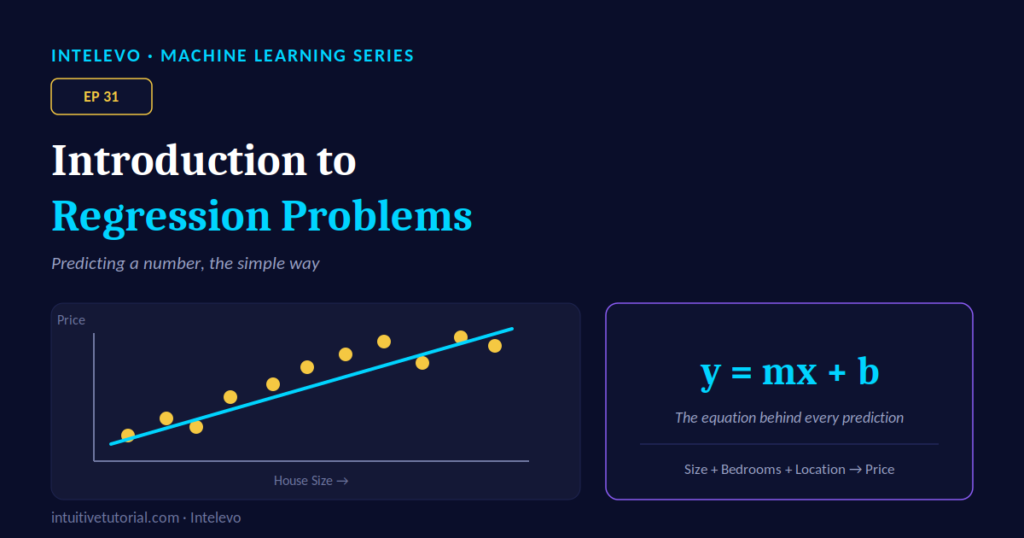
Imagine every house in our dataset becomes one dot on a chart. House size sits along the bottom axis. Price sits along the side axis. Once you plot enough houses, a pattern emerges: as size increases, price tends to increase too.
Regression’s entire job is to draw the straightest possible line through that pattern. This line is called the best-fit line. It represents the model’s best guess at how size and price relate to each other.
Once that line exists, predicting a new house’s price becomes almost effortless. You simply find the house’s size on the bottom axis, trace up to the line, and read off the predicted price.
The Simplest Version of the Idea
Here’s the one formula you actually need to understand regression at its core:
y = mx + b
That’s it. This is simply the equation of a straight line, and it’s the engine behind simple linear regression.
Let’s break down each part in plain words:
- y is the price we’re predicting.
- m is the slope — how much the price rises for every extra square foot.
- x is the house’s size, our input feature.
- b is the intercept — the starting price when size equals zero. Think of it as a mathematical anchor point.
So, in plain words, regression means finding the best possible values for m and b. These values make the line pass as close as possible to every dot on the chart.
Once you know m and b, you can plug in the size of any brand-new house. Then, you can instantly calculate a predicted price. No guesswork required.
Types of Regression, At a Glance
This core idea comes in a few different flavors, depending on how many clues you use and how the pattern bends.
- Simple linear regression uses one feature to draw one straight line. For example, size alone predicts price.
- Multiple linear regression uses several features to still draw one straight line. For example, size, bedrooms, and location together predict price.
- Polynomial regression lets the line bend into a curve. This flavor works well when the pattern in your data isn’t perfectly straight.
However, here’s an important warning. Logistic regression has the word “regression” right there in its name. Despite that, it actually predicts categories, not numbers. So, it belongs to the classification family, not the regression family. This mix-up trips up plenty of beginners, so keep it in mind.
How Do We Know the Guess Is Good?
No line passes through every single dot perfectly. That’s completely normal and expected. The small gap between a house’s real price and the line’s predicted price has a specific name: the error, or the residual.
So, what’s the actual goal here? A good regression model keeps these gaps as small as possible. Importantly, it does this across every house in the dataset, not just one lucky example.
Turning Gaps Into One Score
Once you have all these little gaps, how do you turn them into one overall quality score for your model? Three common metrics answer this question.
MAE (Mean Absolute Error) calculates the average size of the gaps, while ignoring their direction. It’s simple and easy to interpret.
MSE (Mean Squared Error) squares each gap before averaging. As a result, it punishes bigger mistakes far more heavily than smaller ones.
RMSE (Root Mean Squared Error) takes the square root of MSE. This brings the score back into the same units as your target variable, like dollars. Consequently, it’s often the easiest of the three metrics to interpret at a glance.
You’ll rarely calculate these formulas by hand. Instead, one line of Python code gives you every score instantly. What matters most right now is this simple rule: smaller scores always mean a better-fitting model.
Here’s a quick way to build intuition. Suppose our model predicts a house at $300,000, but the real price turns out to be $310,000. That gap of $10,000 is one single residual. Now, imagine calculating that same gap for every house in your dataset, then averaging the results. That average is essentially what MAE gives you, in plain terms. MSE and RMSE simply adjust how heavily large gaps get weighted in that average.
Let’s Predict a Price in Code
Theory is helpful, but code makes everything real. So, let’s build an actual regression model using Python and scikit-learn.
from sklearn.linear_model import LinearRegression

# size (sq ft) and known prices
size  = [[850], [1000], [1450], [1800], [2200]]
price = [180000, 210000, 268000, 310000, 365000]

model = LinearRegression()
model.fit(size, price)

# predict a brand-new house
new_size = [[1600]]
predicted = model.predict(new_size)

print(predicted)   # [289450.]
Let’s walk through this step by step. First, we import LinearRegression from scikit-learn’s linear model module. This class does all the line-fitting math for us.
Next, we set up our data. The size list holds five known house sizes, in square feet. The price list holds the matching known prices for those same five houses.
Then, we create the model with LinearRegression(). After that, we call model.fit(size, price). This single line searches for the best possible values of m and b, completely automatically, behind the scenes.
Once the model finishes fitting, we give it a brand-new house it has never encountered before: 1,600 square feet. Notice that we wrap this value in a list of lists, since scikit-learn expects that exact shape.
Finally, we call model.predict(new_size). This function runs the new size through the learned line, and it returns a predicted price of roughly $289,450.
So, just like that, five lines of data and three lines of scikit-learn code produce a working price predictor. That’s genuinely the entire workflow: fit the line on known examples, then predict on brand-new ones.
Common Mistakes to Avoid
Before wrapping up, let’s flag a few traps that catch beginners off guard.
First, the name itself is misleading. “Regression” doesn’t mean going backward in time. It’s simply the statistical term for fitting a line to data.
Second, more features aren’t automatically better. In fact, irrelevant clues can confuse your model, rather than helping it.
Third, watch out for outliers. One unusually priced mansion sitting in your dataset can drag the entire best-fit line off course for every other house.
Finally, remember that logistic regression is the exception to this whole family. Despite its name, it performs classification, not regression.
Quick Recap
Let’s bring everything together in one glance:
| Concept | In Plain Words |
|---|---|
| Regression | Predicting a continuous number, not a category |
| Feature | An input clue used to make the prediction |
| Target | The number we’re trying to predict |
| Best-fit line | The pattern the model learns from the data |
| Residual / Error | The gap between a real value and the prediction |
| MAE / MSE / RMSE | Ways to turn all those gaps into one overall score |
If you remember nothing else from this article, hold onto this table. It’s the exact vocabulary you’ll need for the rest of this regression series.
Frequently Asked Questions
Is regression the same as prediction? Not exactly. Prediction is the broader goal. Regression is one specific technique for achieving it, used whenever the output is a continuous number.
Do I need to know calculus to understand regression? No. As this article shows, you can understand the entire concept using one simple formula, y = mx + b, and a single visual chart. Calculus becomes useful later, once you start optimizing more complex models.
Which regression type should I learn first? Start with simple linear regression. It uses just one feature, so it’s the easiest way to build genuine intuition. From there, multiple linear regression and polynomial regression will feel like natural extensions, not brand-new topics.
Can regression handle categorical features, like a neighborhood name? Yes, but not directly. You first need to convert categories into numbers, using a technique called encoding. We covered this exact topic in an earlier episode of this series.
What’s the difference between error and residual? In practice, these terms get used interchangeably. Technically, residual usually refers to the gap on data the model was trained on. Error often refers to the gap on brand-new, unseen data.
What’s Next?
Now that you understand the theory behind regression in machine learning, it’s time to build one from scratch. In Episode 32, we’ll take today’s y = mx + b idea and code it ourselves, without relying on any shortcuts or libraries. You’ll write the underlying math in plain Python before ever touching scikit-learn again.
Want to see all of this explained visually, with the same house-price example brought to life on screen? Watch Episode 31 on the Intelevo YouTube channel. Then, subscribe so you don’t miss Episode 32.
Got questions about regression? Drop them in the comments on YouTube. We read every single one.