Introduction
Bandit problems are the simplest possible reinforcement learning scenario. Here the bandit machine can have k arms and pulling each arm leaves the user a reward. One of the arms will be giving higher rewards in the long run and moreover this pattern could be changing over a time period. Think of the scenario of advertisements placed in a website. If the reward can be whether a user clicks on the ad or not, the challenge before the engineering team would be to find the advertisement that leads to more user clicks and hence revenue. Epsilon-greedy algorithm can be used in such a scenario.
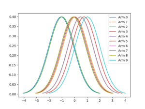
Distribution of k arms

For the purpose of demonstration, lets assume the mean values of arms and individual values are generated from a normal distribution. There are ten arms (0-9) in this Bandit.
Epsilon-Greedy Algorithm
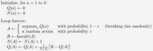
Epsilon-Greedy algorithm is one of he basic algorithm to tackle this problem. In this article we will be trying to implement the same. At any point of the time the agent has to face the exploration-exploitation choice, i.e. to pull an arm that gave a higher reward or try a new arm. In epsilon-greedy this is achieved with a probability value epsilon. If the value of ϵ is 0.2, the agent will pull a random arm 20% of the time and will pull the arm which gave maximum reward 80% of the time. The Psuedo code of the algorithm is shown below.

Code
import numpy as np
import matplotlib.pyplot as plt
import scipy.stats as stats
import math

class Bandit(object):
	def __init__(self, epsilon):
		self.arms = 10
		self.means = np.random.normal(0,1,10)
		self.qvalues = [0]*10
		# self.armcounts = [0]*10
		self.epsilon = epsilon
		self.stepsize = 0.1

	def pullArm(self,arm):
		return np.random.normal(self.means[arm],1,1)[0]


	def plot(self):
		i=0
		for mu in self.means:
			sigma = math.sqrt(1)
			x = np.linspace(mu - 3*sigma, mu + 3*sigma, 100)
			plt.plot(x, stats.norm.pdf(x, mu, sigma), label = 'Arm '+str(i))
			i+=1
		plt.legend()
		plt.show()


def simEpsGreedy(timesteps = 1000, episodes=200, epsilon = 0.1):
	srewards = []
	for episode in range(episodes):
		rewards = []
		np.random.seed(episode)
		myBandit = Bandit(epsilon)
		for timestep in range(timesteps):
			if np.random.random()< myBandit.epsilon:
				arm = np.random.randint(0, myBandit.arms)
				# print('Arm selected Random:', arm)

			else:
				arm = np.argmax(myBandit.qvalues)
				# print('Arm Selected Greedly:', arm)
			# Optional if using stepsize manually
			# myBandit.armcounts[arm]+=1
			# step_size = 1.0/myBandit.armcounts[arm]
			r = myBandit.pullArm(arm)
			rewards.append(r)
			myBandit.qvalues[arm] = myBandit.qvalues[arm]+myBandit.stepsize*(r-myBandit.qvalues[arm])
		srewards.append(rewards)
	srewards = np.mean(np.array((srewards)), axis=0)
	return srewards


for eps in [0.01, 0.1, 0.5]:
	timesteps=600
	final_rewards = simEpsGreedy(timesteps= timesteps, epsilon = eps)
	# final_rewards = np.convolve(final_rewards, np.ones((20,))/20, mode='same')
	plt.plot(range(timesteps), final_rewards, label = 'Eps ='+str(eps))
plt.legend()
plt.show()
Rewards

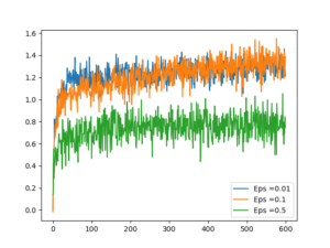
We can see the agent explores first and settles down after sometime, generating highest rewards possible.
The Role of ϵ
As we can see here an ϵ value of 0.1 does better than both 0.5 and 0.01. This is interesting. May be it is because of the number of arms in Bandit. I wonder whether there is any theoretical explanation for this.
