Linear regression is one of the algorithm machine learning enthusiasts start to learn first. In this article, l will walk you through the linear regression intuition. We will implement the basic form of it without using any machine learning packages.
The main philosophy of supervised machine learning algorithms is to learn from data. The algorithms detect patterns in data and use it to build a mathematical model. With such models, we can make better predictions and inferences scientifically. Linear regression is one such technique.
A simple real-life dataset
Let us take a simple dataset (Cricket Chirps Vs. Temperature) from “The Song of Insects by Dr.G.W. Pierce, Harvard College Press”. If you are wondering how does this sound like play the audio below.
The following table represents the data values taken from https://college.cengage.com/.
Visualize the data
We can plot the data to inspect whether there is a correlation between the two variables. The following code does that.
# import some non-ml libraries
import pandas
from matplotlib import pyplot

# set values for clean data visualization
labelsize 	= 12
width 		= 4
height 		= width / 1.618

pyplot.rc('font', family='serif')
pyplot.rc('xtick', labelsize=labelsize)
pyplot.rc('ytick', labelsize=labelsize)
pyplot.rc('axes', labelsize=labelsize)
fig1, ax 	= pyplot.subplots()
fig1.subplots_adjust(left=.16, bottom=.2, right=.99, top=.97)

# read the data
data 		= pandas.read_csv('Temp_Vs_Chirp.csv')

# plot the data
pyplot.scatter(data['Temperature'], data['Chirps'], color ='k')
pyplot.xlabel('Temperature in Fahrenheit')
pyplot.ylabel('# of chirps/sec')

# save the graph
fig1.set_size_inches(width, height)
pyplot.savefig('tempVChirpScatter.jpeg', dpi = 100)
pyplot.close()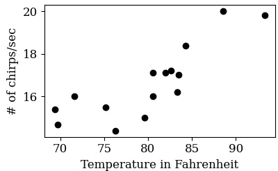
We can see that there is a correlation between temperature and the number of chirpings/sec. As temperature rise, the chirping rate also increases. Now the question is, can we build a model that can predict the chirping rate given a temperature value ?.
Few candidate functions
We can use a mathematical function that roughly represents the data. This way, given a temperature value that is not in our data table, we can find an approximate chirping rate.
One important thing to be considered here is that there could be multiple functions/hypotheses that can approximate the given data. This brings up the question, which one to choose?. The following figure shows how few candidate functions can represent the chirping data.
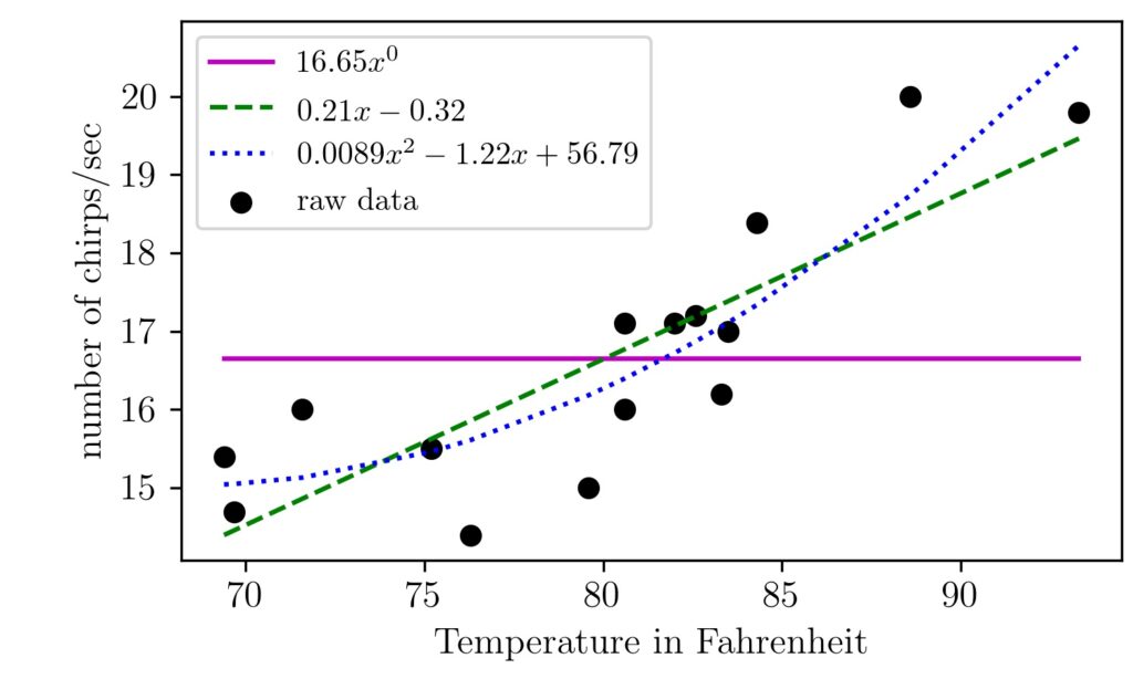
As you can see here, I have shown you three functions ($16.65x^0, 0.21x-0.32, 0.0089x^2- 1.22x+ 56.79$) that can represent the chirping data. I have used a polynomial fit to generate the functions and figures.
The first one here is $16.65x^0$ which is same as the floating point number 16.65, as $x^0$ is 1. This is just the mean value of the number of chirping/sec data we have. Check it out the other article I have written about the mean value.
This number (16.65) here is just a single representative of the chirping data we have over different temperature levels. We can see the mean value (purple line) as the simplest approximation here. As we can see first-order and second-order polynomials capture the data trend better.
A word of warning
However, there is one catch here. Here the polynomial is our model. The complexity of the polynomial will be the number of higher-order terms in it. If we keep increasing the complexity of our model, it will start to get more precise about representing the data we have but fail miserably to the unseen data.
As we start fine-tuning it in a region of interest, it will start to go off wildly in other areas. So the idea here is to select a model that gives us a satisfactory approximation for both seen and unseen data. This is why the training and testing phase in machine learning exists.
Another important idea here is that we don’t know the exact biological/ecological/physical/mathematical relationship between temperature and chirping rate. It could be a complex process with thousands of parameters affecting it. We just know there is some pattern (correlation here) between these variables. So the question here is, does it have any practical value in finding such patterns which are approximate only?.
The answer is YES. As the use-cases become complex with high dimensional data, they often perform better than human beings. Such machine learning algorithms are nowadays part of our life. They translate languages, recognizes speech, drives cars, recommend products for you, etc.
In supervised ML, we often have to make the initial hypothesis about the function. Once it is done, then the next step is what will be the parameters of it so that it approximates best for both seen and unseen data.
Training the model
For the time being, let’s work with the training data. I am going to take the first-order polynomial as the proposed hypothesis function.
It is of the form $mx^1+x^0c$, where $m$ is the coefficient value of the term $x^1$, and c is that of $x^0$.
For a given $m$ and $c$ values, we need to see how our solution is compared the actual data. We need some measures to compare the answers given by our solution to the actual data points we have.
Cost function
The easy way to check it would be to take the difference between the two. Therefore for each point, we have a temperature value predicted by our algorithm and the real temperature value according to our dataset. Likewise, since we have 15 values, we can sum these to come up with a single performance indicator.
Mathematically it can be represented as $ \sum_{i=0}^{15}y_i-(mx_i+c) $. Such measures are often called cost and such mathematical expressions are called cost function in general. The better our hypothesis function, the less cost value will occur. The more our candidate solution deviates from original output values, the higher the cost becomes.
Before proceeding further lets have a visual intuition about the present cost function.
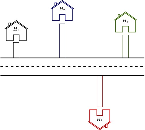
Suppose there is a road to be built passing nearby a colony of houses. For simplicity, we are assuming here that the road has to be straight and not curvy. The pictures below shows a few options we have.
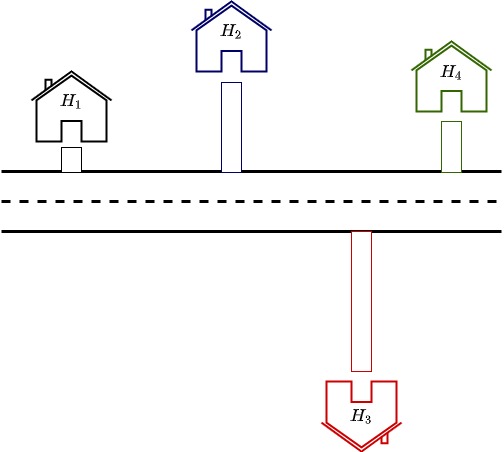
As you can see here houses $H_1$, $H_2$, and $H_4$ are relatively closer together. Or rather the road is built in such a way that it passes nearby $H_1$, $H_2$, and $H_4$. Owner of $H_3$ might be quite unhappy about this and might be looking like a construction shown below.
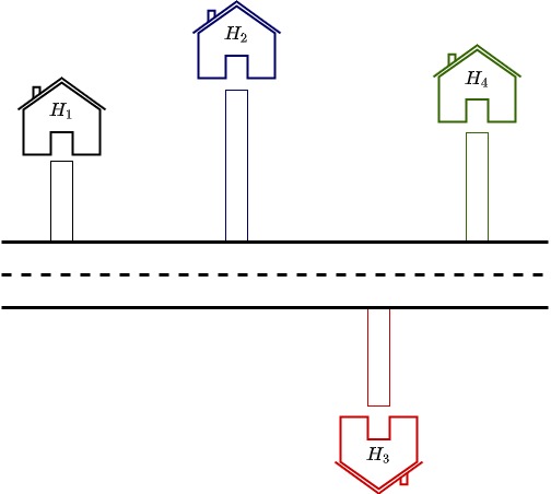
Now the road is closer to $H_3$ but $H_1$, $H_2$, and $H_4$ have to suffer for this. What an ideal solution might be the straight line distance from each house to the road is minimized so that no house is given additional weightage or preference. This is shown in the picture below.
Similarly, when we take the difference between our approximation function and output for test data points, we are trying to minimize the distance in each case. Our cost function in the example was $ \sum_{i=0}^{15}y_i-(mx_i+c) $.
One drawback of this present function is that when we sum these distances together as some of them are positive and some negative, there is a chance for the result to go zero but still it is being a bad fit. To account for this, before summing, the square of the deviation is taken. Now the cost function becomes $ \sum_{i=0}^{15}(y_i-(mx_i+c))^2 $.
This measure is popularly known as Mean Square Error (MSE). You might be thinking, why squaring?. Why not take absolute value/cubic/$n$th power?. The added advantage of squaring includes, it magnifies small and large deviations in a non-linear way, makes the cost function a smooth one, etc. The smoothness helps us to find the appropriate parameter values ($m$ and $c$ here) using approximation methods.
Coming back to the function approximation, now we have a mechanism to check how good a given set of parameters are in constructing the target function. We can assume values for $m$ and $c$ and check the cost associated with it.
Another important point here is that it might look easy to check all possible combinations of $m$ and $c$ and find those values that give the least cost value. This is not as easy as it sounds. Finding the solution by Bruteforce methods quickly becomes intractable as the number of parameters grows. This is known as the Curse of dimensionality.
This is where the approximate solution methods like gradient descent come in. The key idea here is to start with an initial guess for parameter values, observe the cost it is resulting, and make an educated guess on how to change the values of parameters.
It is analogous to tuning a radio. The optimal parameter value is the station frequency. We use the information from the cost (acoustic noise) to determine whether to increase or decrease the tuning frequency value.
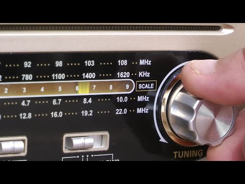
In the radio, it is only one parameter and is a single dimension. In our cricket chirping example, we have two parameters to optimize, and is two dimensional.
How can we incorporate the tuning process algorithmically or programmatically? This is where the idea of Gradient descent comes in.
Gradient descent
To understand this first, we need to know what derivatives and gradients are. For a quick intuition for derivatives let’s take a look at the following figures.
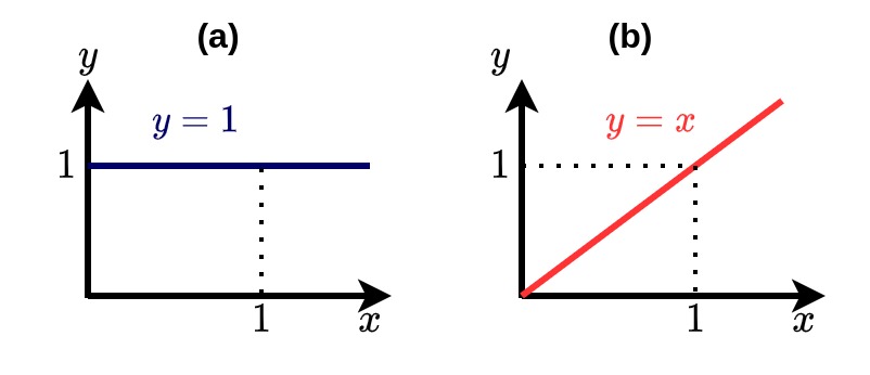
These are two simple functions $f_1$ which is $y=1$ and $f_2$ which is $y=x$. We know that derivative is rate of change of one variable with respect to another. We know the derivative of $f_1$ is zero because no matter whatever change happens to $x$, $y$ remains to the constant value of 1. For $f_2$ the change in $y$ is proportional to the change in $x$. This proportionality constant becomes the derivative, which is equal to 1.
Now the key question here is, Can we say by only looking at the derivative whether the function is increasing or decreasing?. The answer is Yes. The positive derivative value says the fuction is increasing. A negative derivative denotes the function is decreasing. A zero value for derivative appears whenever the function remains same at any point.
The Idea of Abstract Direction
The ideas of abstract direction and vector comes here. You can read more finer details about abstract direction and vectors here. A derivative points towards a direction of maximum increase for the function value. $f_1$ here is always stays same and no increase anywhere. Hence its derivative is also zero. For $f_2$ derivative is a positive value of 1 which means when $x$ increases $y$ increases and when $x$ decreases $y$ also decreases.
Our cost function has two variables $m$ and $c$. This means we need to take the partial derivatives w.r.t both $m$ and $c$. This means we will get a pair of derivatives and it is called a Gradient.
Now given a starting value for $m$ and $c$ we can use the negative of gradient to change the parameters so that the cost is reduced. This is done as tiny steps as the gradient magnitude is normalized using a constant value called learning rate. This is performed as an iterative process until the cost has been reduced to an acceptable low threshold. Lets see how we can implement these programatically.
Code
The first step is to load the data.
</p>
import numpy as np
import matplotlib.pyplot as plt

# read the data
data 		= 	pandas.read_csv('Temp_Vs_Chirp.csv')
x  			=	data['Temperature']
y 			=	data['Chirps']
<p>
The cost function we are going to take is Mean Square Error (MSE).
$ \theta = MSE = \frac{1}{N}\Sigma(y-\hat{y})^2$
Here the variable $\hat{y}$ represents the values predicted by our proposed model. The above formula is the same as shown below after expansion.
$ \theta = MSE = \frac{1}{N}\sum_{i=0}^{N-1} (y_i-\hat{m}x_i-\hat{c})^2$
The derivative of cost function with respect to ${\hat{m}}$ and ${\hat{c}}$ will be different.
$$\frac{\partial \theta}{\partial \hat{m}} = \frac{-2}{N}\sum_{i=0}^{N-1} (y_i-\hat{m}x_i-\hat{c})x_i$$
$$\frac{\partial \theta}{\partial \hat{c}} = \frac{2}{N}\sum_{i=0}^{N-1} (y_i-\hat{m}x_i-\hat{c})$$
So the gradient would be a vector and the negative of that will point to the direction of maximum descent.
$$\Bigg(- \frac{\partial \theta}{\partial \hat{m}}, -\frac{\partial \theta}{\partial \hat{c}}\Bigg)$$
Now we will start with a random guess for $m$ and $c$ and a learning rate small enough.
</p>
import random
alpha = 0.001
mhat = random.uniform(-1, 1)
chat = random.uniform(-1,1)
<p>
Now we will update the estimates of $m$ and $c$ according to the gradient.
$$\hat{m_{new}} = \hat{m}-\alpha \frac{\partial \theta}{\partial \hat{m}}$$
$$\hat{c_{new}} = \hat{c}-\alpha \frac{\partial \theta}{\partial \hat{c}}$$
The values of both partial derivatives (i.e. gradient) forms the abstract direction we were discussing about and will push the values of $m$ and $c$ to a direction so that the cost value is reduced as much as possible. This process is done iteratively till an acceptable low cost value reaches. The following code does that.
</p>
errorsig = []
for i in range(1000):
    cost = np.sum((y-yhat)**2)/N
    partial1 = (-2/N)*np.sum((y-yhat)*x)
    partial2 = (2/N)*np.sum((y-yhat))
    gradient = np.array((partial1, partial2))
    gradient = gradient - gradient.mean()
    gradient = gradient/gradient.max()
    mhat = mhat - alpha*gradient[0]
    chat = chat - alpha*gradient[1]
    yhat = mhat*x+chat
#     plt.scatter(x,y)
#     plt.plot(x,yhat)
#     plt.savefig('Animations/anim'+str("{0:0=4d}".format(i))+'.png')
#     plt.cla()
    errorsig.append(cost)
<p>
I have turned off the visualization but you can uncomment that and it will save a series of images after each iteration. These images shows us how the slope $m$ and $y$ intercepts are dynamically changes so that cost value goes down as little as possible. Following video shows the animated dynamics of the same.
Finally lets printout the cost value and estimated parameter values of our model.
</p>
print(cost, mhat, chat)
<p>
I am getting 0.81, 0.20, 0.04 respectively. This is different but close to the parameter values we got from polynomial fit. Smart optimization techniques can make the training process faster and accurate. Once the parameter values are found, we can use them to predict cricket chirps for different temperature values.
Pingback: K-Nearest Neighbors Algorithm - Intuitive Tutorials