Overview
In this note about distributional reinforcement learning, I am going to reflect on the paper titled A Distributional Perspective on Reinforcement Learning. I will try to give an overview of the underlying ideas behind this paper. Please keep in mind that a research contribution is often a culmination of multiple ideas/components. This makes from the scratch tutorial/explanation of research papers lengthy and difficult. Still, I want to give it a try and see how far I can get.
This paper comes from the subject area of reinforcement learning (RL). The whole idea of learning algorithms is reshaping our day to day life. Supervised machine learning algorithms, especially deep neural networks made a huge splash in the tech industry. Although not as popular as supervised learning methods, reinforcement learning algorithms are considered in the journey towards artificial intelligence.
This is because unlike supervised learning, the guiding principle behind RL is not learning from examples but learning from trial and error. You might be wondering what is the difference between the two. Isn’t it supervised learning is also learning from trial and error?. aren’t we using training, error minimization, etc?.
The key difference is whether an algorithm use data that were annotated or labeled by humans. A neural network model needs access to human-labeled data to get trained so that it can classify an image as a cat or dog. If you observe closely in our real-life we never learn in a supervised learning setting. We all learned to walk. Nobody told us what to do in every situation like how to climb steps, what to do when you slip, on what angle we should place the foot, etc. It was all trial and error. But we all have access to the environment in which we were able to interact and get feedback. It is this philosophy that reinforcement learning algorithms follow.
The philosophy of RL says out loud that we only need access to the reward signal to learn from the environment. This might seem counter-intuitive to the fact that we learn more in presence of uncertainty. I remember some psychological studies that prove we learn more while we make mistakes than getting it right. This is sort of analogous to from an information-theoretic point of view. The information content is higher when there is more uncertainity.
Distributional Reinforcement Learning
Despite all this chaos, the distributional reinforcement learning (DRL) takes a direction against the flow of conventional theory. This is where things get interesting. In DRL instead of the sparse rewards, the distribution of rewards are processed and it performs better too.
The key idea of the paper is the argument that rather than the value function, the value distribution is important in reinforcement learning and leads to better results. The conventional RL uses the expected value of return at a given state while the Distributional RL considers the distribution of the same. You can read about these introductory concepts here. The authors of DRL paper have defined value distribution as the distribution of random return received by the reinforcement learning agent.
The authors state that there is an established body of literature studying the value distribution but focuses on implementing risk-aware behavior. They claim to provide theoretical results in policy evaluation and control. This is further supported along with empirical evidence. The authors admit that there is some instability in the policy control part, the reason for the same is not clear though.
Introduction
The introduction starts with the traditional Bellman equation of value. In RL, Unless otherwise constrained in its behavior an agent is supposed to maximize this Q value. The equation for the Bellman action-value is given.
$Q(x,a) = \mathbb{E} R(x,a)+\gamma \mathbb{E} Q(X’, A’)$
The equation means the action-value of a state $x$ taking an action $a$ will transform the agent to another state $X’$ at where it can take another action $A’$. The action-value is the sum of the immediate reward plus the discounted sum of future action-values.
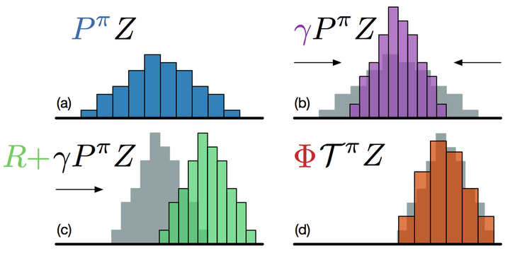
Now what they are proposing is to forget about taking the expectation but consider the resulting distribution. This is denoted by the second equation which is copied below.
$$Z(x,a) \stackrel{\mathrm{D}}{=} R(x,a)+\gamma Z(X’,A’),$$
This is called the distributional Bellman equation. The authors state that this $Z$ is characterized by the interaction of three random variables: the reward $R$, next state-action $(X,A’)$, and its random return $Z(X’,A’)$.
The distributional perspective is old as the Bellman equation itself. But so far it has used for other purposes like modeling parametric uncertainty, designing risk-sensitive algorithms, or for theoretical analysis. This is where the authors use it for much important purpose.
One important point to note here is that the Bellman equations work due to the Contraction property it has. Because of the case, changing value function to distribution also has to follow such characteristics so that the value distribution will converge. For this to happen, a metric called Wasswestein is used based on some previous studies.
When it comes to policy control and Bellman optimality, this contraction property does not work as it is. Like in value functions we need to compare different action-values to update policy. The distributional analogous here would be something like Wasserstein metric I guess.
The benefits of learning approximate distribution are mentioned next. One is the multimodality of the distribution is preserved, mitigates the effects of learning from a non-stationary policy. They argue that their method gives an increased performance in Atari 2600 games. One point to note here is that it does not achieve a state of the art performance in all games but in some.
Reflections from Discussion
The discussion part elaborates why value distribution matters. The authors say that the value distribution is important in the presence of approximation. It also helps to reduce the effect called chattering while using function approximation cases. It helps to mitigate state aliasing effects. They touch upon the importance of choosing the metric (KL divergence or Wasserstein) to optimize.
Concluding Remarks
I think the paper is well written setting up a new possibility in RL altogether. The code of the algorithms they proposed (C51) is available. The cited papers also seem interesting. As of today, C51 has become one of the standard RL algorithms. There have been some follow-up works that build upon the fundamentals raised by this DRL paper.