This post is a case study on primary or metastasis classifier using deep learning models.
Overview
Genetics is behind every physiological aspect of a living being such as height, eye color, hair color, etc. Mutations are unwanted changes happening to genetic code for various reasons. The main reasons account for such changes are hereditary, exposure to environmental radiation, and errors that occur in DNA replication. Some of these mutations alter the behavior of human cell growth in a harmful way causing tumor growth and thereby called the disease Cancer. Cancer is a disease in which cells in the human body grow uncontrollably. This becomes life-threatening as the disease progresses through various stages.
Business Problem
Modern gene sequencing technologies are getting cheaper year after year and also generate huge amounts of genetic data. With deep learning techniques, it is possible to build an early diagnosis and prognosis solution that can predict whether a particular genetic mutation is of type primary or metastasis. In this work, with the deep learning model, I will be predicting whether a given mutation is primary or metastasis. To accomplish this task novel deep learning algorithms and architecture will be applied on clinical research data. This will help to benchmark this study with related studies. Also since the application of the technology for this objective is first to the best of our knowledge, the research findings will add value to the scientific community as well as act as pilot study proving the business value.
Business Constraints
The business constraints start with the feasibility and availability of mutation data. To generate mutation data for diagnostic purposes, it is required to do Whole Genome Sequencing or Whole Exome Sequencing, whose costs are decreasing year after year but adoption of such technologies are rather happening slowly. The other major constraint is that prediction from the model needs to be validated by a qualified oncologist who will be the end user of the model, so that he/she can plan further therapeutic plans. When it comes to commercial deployment of the application. The whole prototype needs to be examined and approved by respective agencies (subject to countries) like Food and Drug Administration (FDA). Also ethical and data privacy considerations have to be taken care of when implementing it as a business solution.
Dataset
The major dataset used in this study is coming from state of the art open clinical research data called Memorial Sloan Kettering-Integrated Mutation Profiling of Actionable Cancer Targets (MSK-IMPACT). It is open research data available from a platform called CBioportal. CBioportal is an open access resource for interactive exploration of multidimensional cancer genomics data sets. CBioportal hosts data from large consortium efforts, like TCGA and TARGET, as well as publications from individual labs.
Performance Metrics
The primary performance metric considered will be the accuracy of the model. Other metrics such as sensitivity and Area Under the Curve (AUC) can also be used.
Existing Approaches
Gupta, Prashant, et al. “A new deep learning technique reveals the exclusive functional contributions of individual cancer mutations.” Journal of Biological Chemistry 298.8 (2022).
In this paper the authors have created a Continuous Representation of Codon Switch (CRCS), a deep learning method that allows to generate numerical vector representation of mutations. The CRCS proposed to help them to detect cancer-related somatic mutations in the absence of matched normal samples, enable driver gene identification, and to score individual mutations in a tumor sample. Mutations from healthy individuals are used for learning the vector embedding. The biggest take away from the study is that machine learning models should be created in a chromosome specific manner to enable various genotype-phenotype association studies
Zeng, Zexian, et al. “Deep learning for cancer type classification and driver gene identification.” BMC bioinformatics 22.4 (2021): 1-13.
Genetic information is used traditionally to predict the type of cancer and its sub-types. Somatic mutations are the most frequently used features to predict the cancer type. This paper describes the use of genetic variants including germline variants, and small insertions and deletions for cancer type prediction. The proposed deep learning model is named as DeepCues which is a CNN model that uses whole-exome sequencing data, germline variants, somatic mutations including insertions and deletions for cancer type prediction. The dataset used is from The Cancer Genome Atlas (TCGA) program to classify seven different types of major cancers and obtained an accuracy of 77.6%. Other Than identifying the cancer types, top 20 breast cancer relevant genes are also identified using the proposed model.
Jiao, Wei, et al. “A deep learning system accurately classifies primary and metastatic cancers using passenger mutation patterns.” Nature communications 11.1 (2020): 1-12.
In this study, a deep learning classifier is used to predict cancer types. The prediction is based on patterns of somatic passenger mutations detected in whole genome sequencing of 2606 tumors across 24 common cancer types. The dataset used in the study is Pan-cancer Analysis of Whole Genomes (PCAWG) dataset. The authors report a test accuracy of 91% on held-out test data.
First Cut Approach
The approach planned to solve this problem is as follows. As a preliminary step data will be explored, cleaned, and preprocessed. Extensive Exploratory Data Analysis (EDA) will be carried out to mine insights from the data. This will be carried out with a scientific mindset by posing various questions and analysis will be carried out to find answers to those questions. As the next step, standard correlation analysis will be carried out to measure the predictive nature of various features against the target variable. Those features which have promising correlation to target variable will be further performed with simple statistical tests to identify causal nature of the features.
To come up with novel contributions various DNN architectures will be tried out. Other techniques such as feature engineering and hyperparameter tuning will also be tried out and performance will be compared against the performance reported in the research papers. After necessary modifications, the final model will be created and its performance will be validated against all other models.
Data Preprocessing
The MSK-IMPACT data has multiple files and the important information is spread across multiple files such as ‘clinical data’, ‘clinical patient’, ‘clinical sample’, ‘data mutations’ etc. Basic inspection of these files such as inspecting dimension, column names, and visualizing the first few rows using head commands are done. Important data frames are merged based on relevant common columns and duplicate columns are dropped to avoid redundancy.
Convert Categorical Data Columns to Numerical
A few of the categorical features are easily converted into numerical ones by replacing their content.
data['SPECIMEN_TYPE'].replace(['Resection', 'Biopsy','Cytology','CUSA'],[0, 1, 2, 3], inplace=True)
data['SOMATIC_STATUS'].replace(['Matched', 'Unmatched'],[0, 1], inplace=True)
data['SEX'].replace(['Male', 'Female'],[0, 1], inplace=True)
data['SMOKING_HISTORY'].replace(['Prev/Curr Smoker', 'Never','Unknown'],[0, 1, 2], inplace=True)
data['SampleType'].replace(['FFPE', 'DNA', 'Cell Pellet','FNA', 'Other'],[0, 1, 2, 3, 4], inplace=True)
data['SAMPLE_COLLECTION_SOURCE'].replace(['In-House','Outside'],[0, 1], inplace=True)
data['VITAL_STATUS'].replace(['ALIVE','DECEASED'],[0, 1], inplace=True)
Exploratory Data Analysis
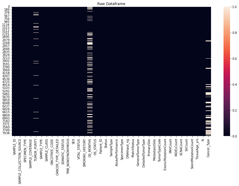
A binary heatmap to visualize missing values is done as the first step in Exploratory Data Analysis.
fig, ax = plt.subplots( figsize = (15, 8))
sns.heatmap(data_table.isnull())
ax.set_title('Raw Dataframe')
plt.show()
Inorder to quantify the percentage of missing values across features, following analysis is carried out.
total =  data_table.isnull().sum().sort_values(ascending = False)
percent = (data_table.isnull().sum() / data_table.isnull().count()).sort_values(ascending=False)
missing_data = pd.concat([total, percent], axis = 1, keys = ['Count_NaN', 'Percentage_Nan'])
missing_data.head(14)
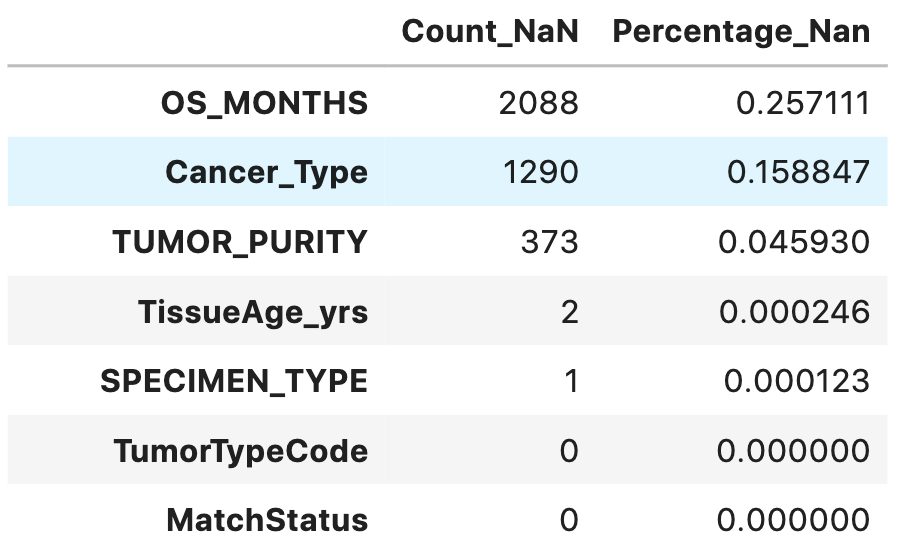
Drop columns having more than 5% of missing values: overall survival months feature and cancer type feature have missing values of 25% and 15%. Hence these features can be removed.
data_table = data_table.drop(['OS_MONTHS',  'Cancer_Type'],axis=1)
# Drop target variable if needed for correlation analysis
master_data = data_table.drop(['SAMPLE_TYPE'],axis=1)
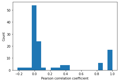
Feature Correlation Analysis
To get an overall idea of correlation between features, the correlation matrix is computed and the same is visualized with the help of histogram and heatmap. Obviously every feature will be correlated with itself with a correlation value of 1. Hence diagonal elements of the heatmap can be ignored.
# Find correlation between features
corrMat = master_data.corr().values
plt.hist(corrMat.flatten(),20)
plt.xlabel('Pearson correlation coefficient')
plt.ylabel('Count')

fig, axs = plt.subplots(figsize = (15, 10))
sns.heatmap(master_data.corr())
plt.title('Correlation between all Features')
plt.show()

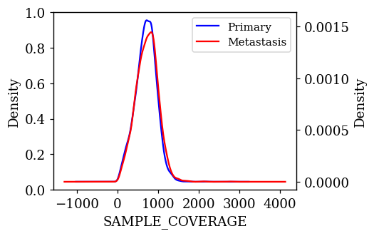
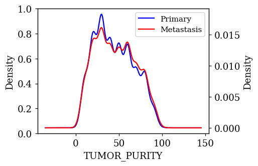
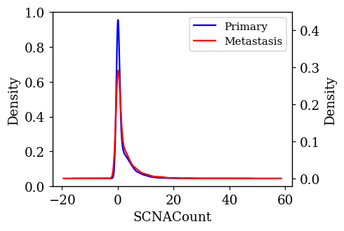
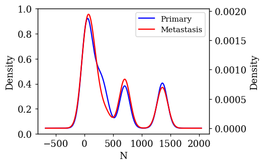
Density Plots of Numerical Features w.r.t Target Variable
The probability density of each numerical feature was computed using Kernel Density Estimation (KDE) with respect to the target variable and is plotted. If a feature is having a decisive role in the classification, then we can expect to see less overlap between the density plots. The KDE plots which are promising and have less overlap are shown below.
Statistical Test on Numerical Features
To statistically assess the significance of a feature to distinguish a mutation as of type Primary or Metastasis, a T-test is performed for each group (Primary and Metastasis).
statDF = pd.DataFrame()
for feature in numericalFeats:
    group1 = data_table[data_table['SAMPLE_TYPE'] == "Primary"]
    group2 = data_table[data_table['SAMPLE_TYPE'] == "Metastasis"]
    tstats, p_value = stats.ttest_ind(group1[feature], group2[feature])
    statDF = pd.concat([statDF, pd.DataFrame.from_records([{'Feature': feature,\
                                                   't-statistics':tstats,\
                                                   'P_value': p_value}])])
The following table shows significant features sorted by P-value in ascending order and marked as significant when the P-value is less than an alpha level of 0.001.
statDF['Significant'] = statDF['P_value']<0.001
statDF.sort_values('P_value')
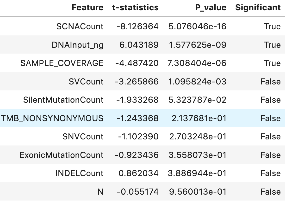
Three statistically significant features SCNACount, DNAInput_ng, SAMPLE_COVERAGE with an alpha level of 0.001 were found out.
significantFeats = statDF[statDF['Significant']==True]['Feature'].tolist()
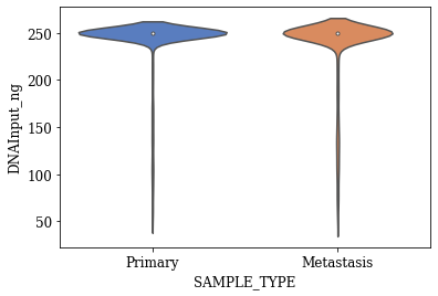
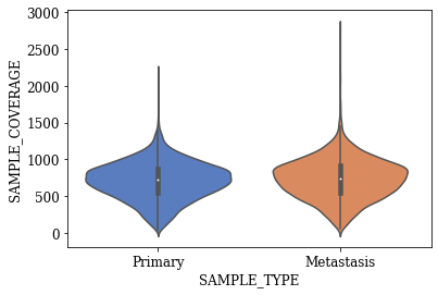
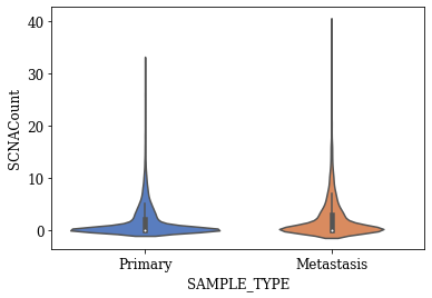
Violin Plots of Significant Features
The violin plot for any feature will show the distribution, its skewness, median values, outliers if any etc. The violin plots created for the statistically significant features found using T-test are shown below.
def myviolinplot(feature, data):
    sns.violinplot(y=feature,\
                   x="SAMPLE_TYPE",\
                   data=data,\
                   palette="muted",\
                   split=True)
    plt.show()

for variable in tqdm(significantFeats):
    myviolinplot(variable,data_table)
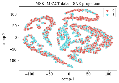
T-SNE Visualization
The T-SNE visualization is done to see if there is any pattern among the two classes of data points primary and metastasis. To do that the target variable is converted into a binary variable from categorical variable and only numerical data is used for T-SNE visualization.
data_table['SAMPLE_TYPE'].replace(['Primary', 'Metastasis'],  [0, 1], inplace=True)
numericalFeats = data_table.select_dtypes('number').columns
categoricalFeats = data_table.select_dtypes('object').columns
numdata = data_table[numericalFeats]
numdata = numdata.fillna(numdata.mean())

tsne = TSNE(n_components=2, perplexity=20.0, n_iter=2000,verbose=1)
z = tsne.fit_transform(numdata)

df = pd.DataFrame()
df["y"] = numdata['SAMPLE_TYPE']
df["comp-1"] = z[:,0]
df["comp-2"] = z[:,1]

sns.scatterplot(x="comp-1", y="comp-2", hue=df.y.tolist(),
                palette=sns.color_palette("hls", 2),
                data=df).set(title="MSK IMPACT data T-SNE projection")
Outlier Analysis
As a next step outlier detection analysis is carried out. To identify outliers, each numerical feature is transformed into its respective z-score. If the absolute value of z-score is greater than 3, then the data point was considered as an outlier.
# Compute Z-Scores
num_zscores = numdata.apply(zscore)

# Find all cells where zscore>3 or zscore<-3
num_zscores_binary = num_zscores.abs()>3

fig, axs = plt.subplots(figsize = (15, 10))
sns.heatmap(num_zscores_binary)
plt.title('Outlier data points across patients |z-score|>3')
plt.show()
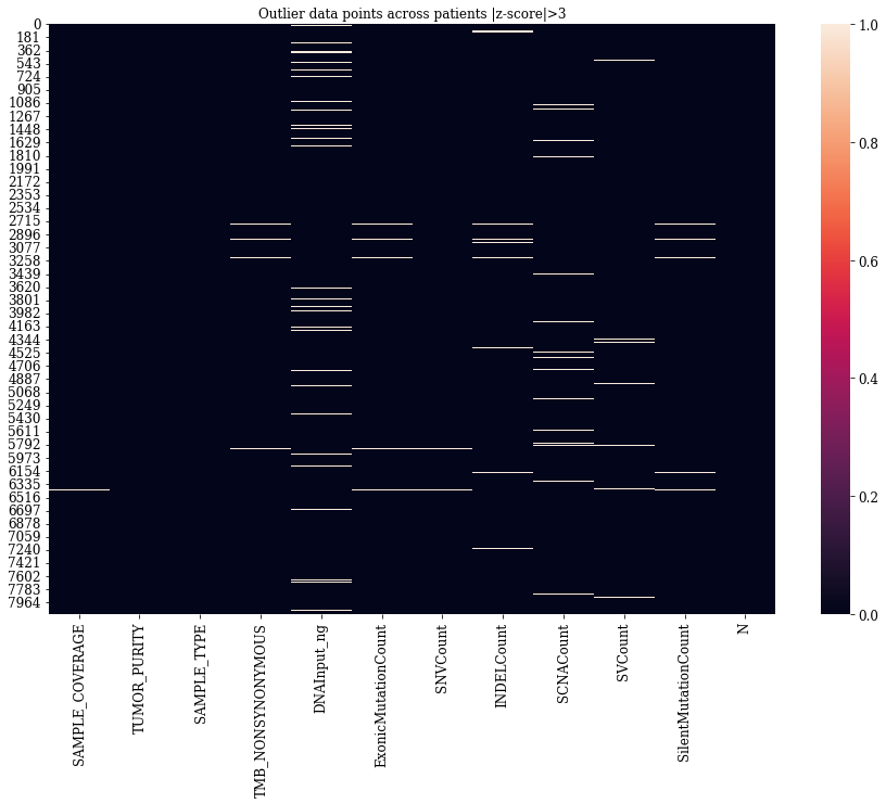
It is observed that the outliers for numerical features are not very much from the heatmap.
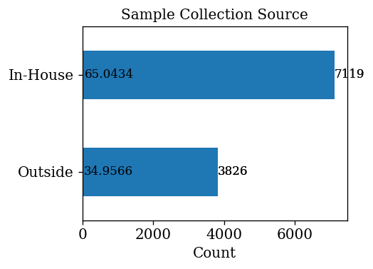
Inspecting Features Manually
Each feature from the combined dataset was plotted with suitable types of graphs and observations are made. The following passage summarizes the findings from plots which are relevant.
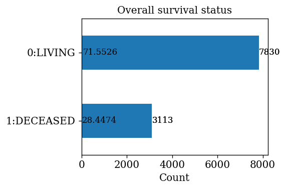
- It can be seen that 71.55% of patients are alive and 28.45% patients are deceased
- 65.04% of samples are collected In-House and 34.96% of samples are collected outside home
- Only one sample is collected from majority (89%) of patients
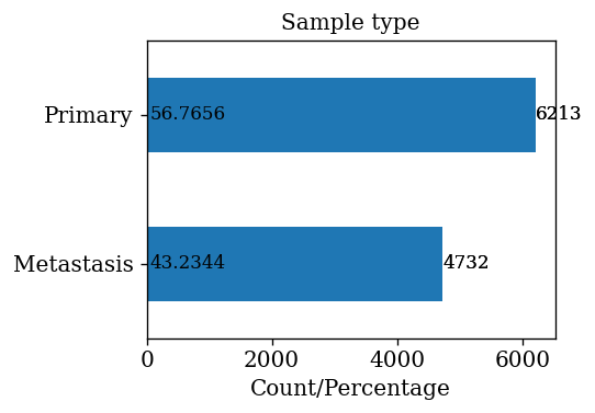
- 43.23% of samples are that of metastasis stage
- Gender distribution of patients is more or less equal (i.e. 50%-50%)
- More than 82% of specimens are preserved as FFPE blocks
- Most frequent codon change is Cga/Tga
- Most frequent class is deletion
- Most frequent connection type is 3to5
- Overall Survival Months feature and Cancer type feature has missing values of 25% and 15%. Hence these features can be removed
- Certain features are highly correlated (both positive/negative correlation with each other)
- Density plots of numerical features between target variable shows some distinction between probability density graphs
- Three statistically significant features ‘SAMPLE_COVERAGE’, ‘DNAInput_ng’, ‘SCNACount’ with an alpha level of 0.001 were found out
- The violin plots of significant features with respect to target variable shows some difference
- There is a good number of outliers (|z-score|>3) among numerical features
- TSNE plot shows some difference/separability between both primary and metastasis classes
Feature Engineering
Few feature engineering steps are done by combining the sample data with mutation data and following mathematical operations are performed on the respective feature.
| No | Feature | Operation |
| 1. | t_ref_counts | Mean |
| 2. | t_alt_counts | Mean |
| 3. | protein_poss | Mean |
| 4. | codon_counts | Len |
| 5. | pos_diffs | Sum |
t_ref_counts = []
t_alt_counts = []
protein_poss = []
codon_counts = []
pos_diffs = []
for sample_id in tqdm(sample_ids):
    segment = data_mutations[data_mutations['Tumor_Sample_Barcode']==sample_id]
    pos_diff = segment['End_Position']- segment['Start_Position']
    pos_diff = np.sum(pos_diff)
    codons  = segment['Codons'].values
    codons = [x for x in codons if str(x) != 'nan']
    t_ref = np.mean(segment['t_ref_count'])
    t_alt = np.mean(segment['t_alt_count'])
    protein_pos = np.mean(segment['Protein_position'])
    t_ref_counts.append(t_ref)
    t_alt_counts.append(t_alt)
    protein_poss.append(protein_pos)
    codon_counts.append(len(codons))
    pos_diffs.append(pos_diff)
Besides this all numerical features are standardized using the Standard Scalar function in Scikit-learn preprocessing.
Primary or Metastasis classifier
Modeling
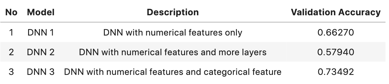
Out of the total data 70% is used for training and 30% for testing. A total of 3 models were tried for this case study, each one is different from the other in certain aspects. The architecture and specification of the models are explained in the coming paragraphs.
Model 1 Architecture
As a baseline a simple Deep Neural Network (DNN) with 7-layers was considered. The following diagram and summary shows the architecture of the DNN used.
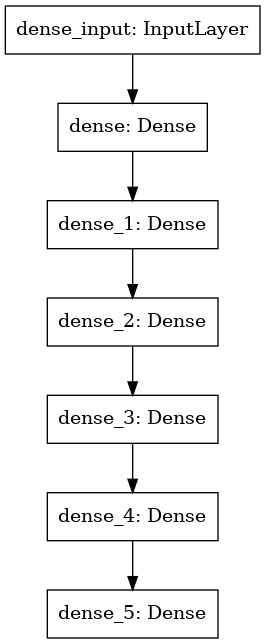
Model 1 Code
model_1 = Sequential()

model_1.add(Dense(64,\
                input_shape=(X_train_num.shape[1],), \
                activation='relu'))

model_1.add(Dense(128,\
                kernel_initializer=RandomUniform(minval=-0.05, maxval=0.05),\
                activation=tf.nn.relu))

model_1.add(Dense (128,\
                 activation = 'relu'))

model_1.add(Dense (64,\
                 activation = 'relu'))

model_1.add(Dense(32,\
                activation='relu'))

model_1.add(Dense(2,\
                activation='softmax'))
Model 2 Architecture
Model 2 is added with more layers as well as dense units. Regularization is added since it has more parameters to train. Model 2 summary is shown below.

Model 2 Code
model_2 = Sequential()

model_2.add(Dense(32,\
                  kernel_initializer=RandomUniform(minval=-0.05, maxval=0.05),\
                  input_shape=(X_train_num.shape[1],),\
                  activation='relu'))

model_2.add(Dense(64,\
                  kernel_initializer=RandomUniform(minval=-0.05, maxval=0.05),\
                  activation=tf.nn.relu))

model_2.add(Dense (128,\
                   kernel_initializer=RandomUniform(minval=-0.05, maxval=0.05),\
                   activation = 'relu'))

model_2.add(Dense (256,\
                   kernel_initializer=RandomUniform(minval=-0.05, maxval=0.05),\
                   activation = 'relu'))

model_2.add(Dense (512,\
                   kernel_initializer=RandomUniform(minval=-0.05, maxval=0.05),\
                   activation = 'relu'))

model_2.add(Dense(128,\
                  kernel_initializer=RandomUniform(minval=-0.05, maxval=0.05),\
                  activation='relu'))

model_2.add(Dense(64,\
                  kernel_initializer=RandomUniform(minval=-0.05, maxval=0.05),\
                  activation='relu'))

model_2.add(Dense(2,\
                activation='softmax'))
Model 3 Architecture
In model 3, detailed tumor type is also added as additional categorical input along with the numerical features. The concatenate function is used to achieve this functionality.
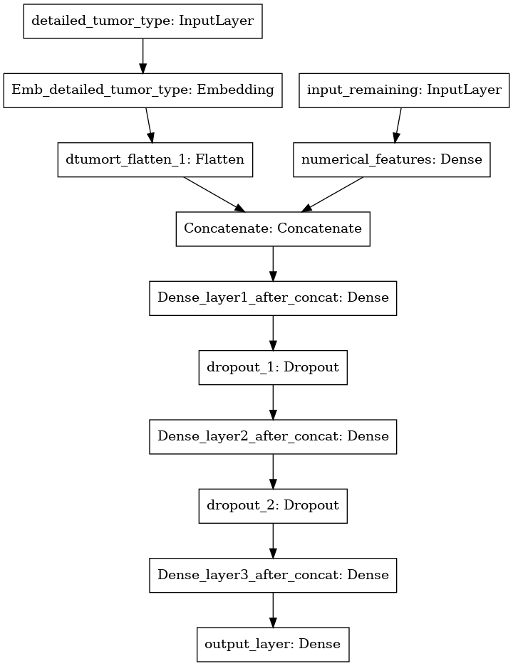
Model 3 Code
tokenizer = Tokenizer()

tokenizer.fit_on_texts(X_train['DetailedTumorType'])
X_train_dtumort = tokenizer.texts_to_sequences(X_train['DetailedTumorType'])
X_test_dtumort = tokenizer.texts_to_sequences(X_test['DetailedTumorType'])
X_train_dtumort = pad_sequences(X_train_dtumort, dtype='uint8')
X_test_dtumort = pad_sequences(X_test_dtumort, dtype='uint8')

num_inp = Input(shape=X_train_num.shape[1], name='input_remaining')
num_dense = Dense(8, activation='relu', name='numerical_features')(num_inp)

dtumort_inp = Input(shape=11, name='detailed_tumor_type')
dtumort_inp_emb = Embedding(input_dim=X_train_dtumort.max() + 1,\
                            output_dim=10,\
                            input_length=5,\
                            name='Emb_detailed_tumor_type')(dtumort_inp)
dtumort_flat = Flatten(name='dtumort_flatten_1')(dtumort_inp_emb )

concat_layer = Concatenate(name='Concatenate')([num_dense,\
                                                dtumort_flat])

dense_1 = Dense(256,\
                activation='relu',\
                kernel_initializer=RandomUniform(minval=-0.05, maxval=0.05),\
                name='Dense_layer1_after_concat')(concat_layer)

drop_1 = Dropout(0.2, name='dropout_1')(dense_1)

dense_2 = Dense(128,\
                activation='relu',\
                kernel_initializer=RandomUniform(minval=-0.05, maxval=0.05),\
                name='Dense_layer2_after_concat')(drop_1)

drop_2 = Dropout(0.15, name='dropout_2')(dense_2)

dense_3 = Dense(64,\
                kernel_initializer=RandomUniform(minval=-0.05, maxval=0.05),\
                activation='relu',\
                name='Dense_layer3_after_concat')(drop_2)

output_layer = Dense(2, activation='softmax',name='output_layer')(dense_3)

model_3 = Model(inputs=[num_inp,\
                        dtumort_inp],\
               outputs=output_layer)
Custom Callbacks
To efficiently train the DNN models a set of custom callbacks have been defined. First one is for early stopping of training when a desired level of validation accuracy (0.95) is obtained. Another one is for the purpose of logging loss, accuracy, validation loss, validation accuracy, and validation f1-score.
Training Settings
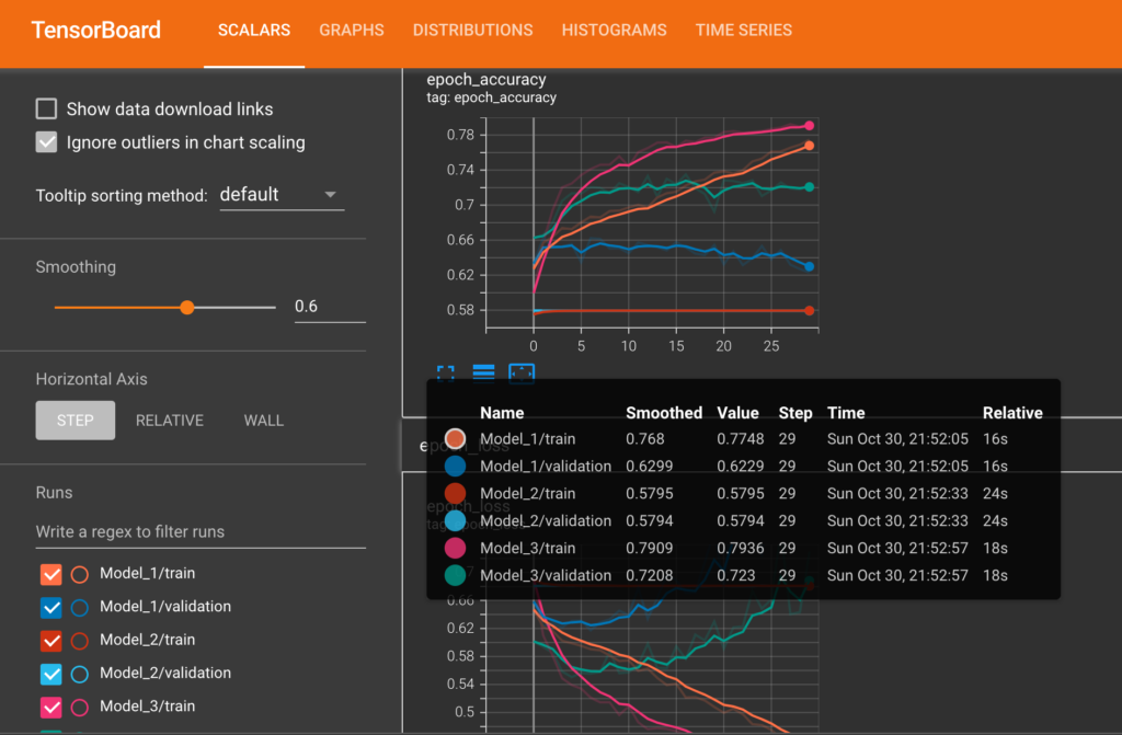
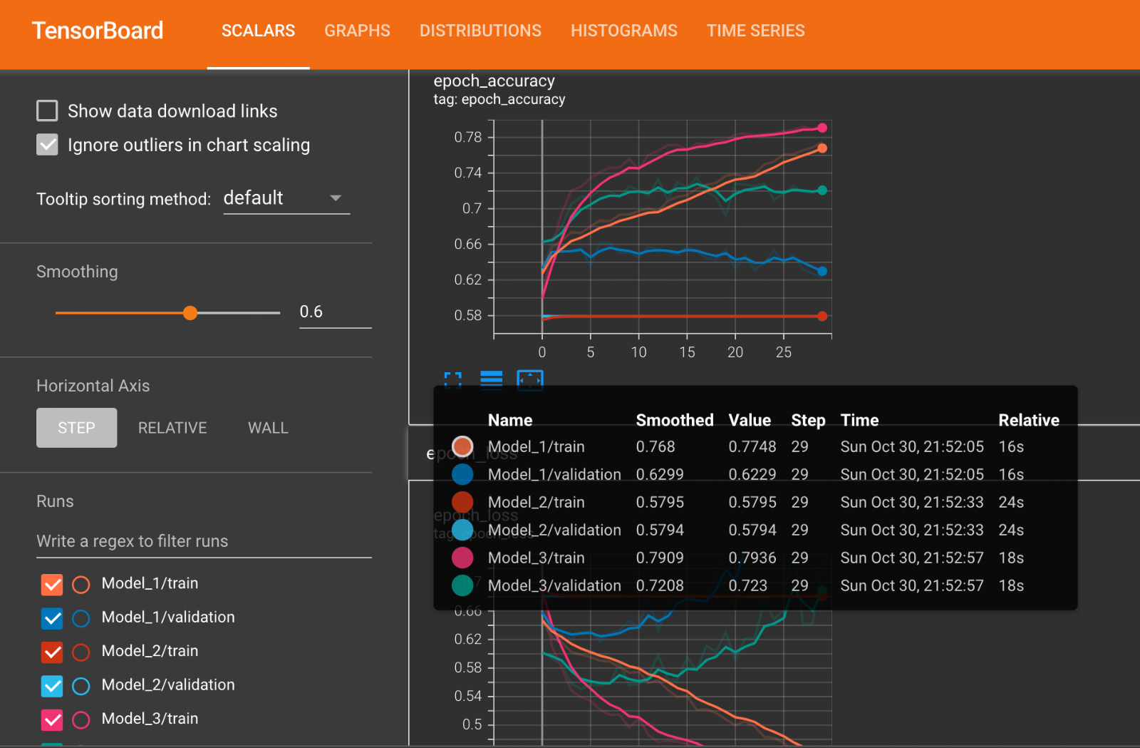
Each model is trained using Adam optimizer with a learning rate of 0.01, batch size of 64, and for a total epoch of 30. All models are checkpointed and saved according to best validation accuracy. Tensorboard is used to visualize the training loss and validation loss of each of the three models.
Results
The performance of all the three models are summarized in the table below. It can be seen that model 3 is having the highest validation accuracy among all other models.
Tensorboard Plots
The following diagram shows train and validation loss & accuracy plots of each of the models from Tensorboard.
Future Work
This current study involves analyzing and predicting mutation data which is available from clinical settings. Future work will include building real-time detection algorithms that can classify primary/metastasis mutations using point care devices.
GitHub Repository
Please find the link to the whole codebase (data preprocessing, EDA, and modeling) in the GitHub repository here: https://github.com/cksajil/OncoMut
Connect with me on LinkedIn here: https://www.linkedin.com/in/sajilck/