What are Support Vector Machines?
Support Vector Machines (SVM) is one of the most elegant methods used for classification and regression in machine learning (ML). We can use SVM when we have a bunch of objects/features which we want to classify.
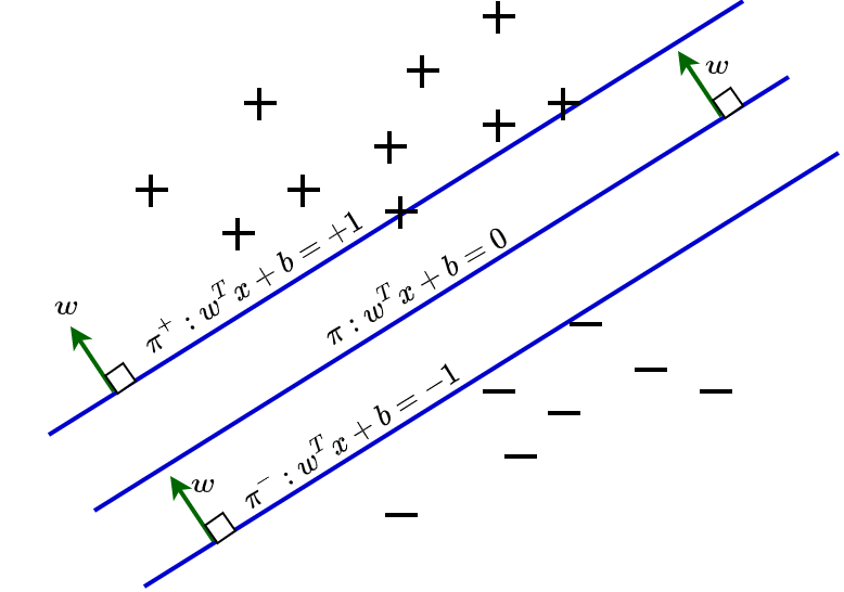
SVM performs the classification by drawing a hyperplane (Figure.1) to separate each category of points belonging to distinct features in n-dimensional space. In two-dimensional space, the hyperplane is a line separating different features and it is a plane separating distinct features in three-dimensional space and so on. SVM tries to find the best plane which gives the maximum distance between points belonging to different categories. The distance to each point from the hyperplane is called a support vector.
Don’t you feel curious to know support vector machines in detail when you realize, this technique can be used for face detection, spam filtering and recognizing handwriting!! Not limited, the applications of SVM extend to gene classification in bioinformatics and to control chaotic dynamics in physics as well.

Methodology
Finding the best hyper plane
The distance between each data point belongs to a class and the hyperplane separating them are called margins. The hyperplane separates the points as demonstrated in Figure.1. We can draw hyperplanes parallel to the separating hyperplane on either side as shown in title figure by choosing it to pass through the immediate data points from the hyperplane. The distance between these two planes ($H^+$ and $H^-$) is called margin. The distance of points lie on $H^+$ and $H^-$ to the margin maximizing (separating hyperplane) are called support vectors. The objective of SVM algorithms is to find the best hyperplane which maximizes the margin. But what if a point belongs to one category goes to the other side of hyperplane containing data points belongs to another category.
SVM consider these points as outlier points and the algorithms in SVM has the characteristic to ignore such outlier points and find the best hyperplane which maximizes margin. We consider a hyperplane as the best hyperplane if the distance of data points on each side from this hyperplane is maximum in comparison with other possible hyperplanes.
Measuring cost of the model
All machine learning models has to be tuned in a way that the loss or cost of the model should be minimum. A cost function is a function represented by specific mathematical formula measures the error rate of the model, which in turn reveals how well the model performs. Some of the well-known cost functions using in classification and regression are Gini impurity and logarithmic loss in classification as well as mean absolute error and root mean square error in regression. Likewise Hinge loss is a cost function specifically engineered to tailor support vector machines.
Minimization of loss by measuring Hinge loss

If there are outlier points after we select a best possible hyper plane, What SVM does is, after selecting the maximum margin, it adds a penalty in the form of hinge loss each time a data point crosses the boundary separating it from the data points belongs to the other class. SVM algorithms tries to minimize $\frac{1}{margin+\Sigma hinge loss}$.
The figure 3 demonstrate the behaviour of hinge loss. The x -axis represents distance of any data point from the boundary separating the correctly classified points from the incorrectly classified points. The y-axis represents the size of loss undergone by the function with regard to its distance.
Before going to the mathematical formulation of hinge loss, let’s understand the behavior of Hinge loss with the aid of the schematic shown above (figure 3).
- The dashed line on the x-axis covers a distance of one unit. It reveals when the distance from the boundary is 1 or greater than 1 unit, the loss function is negligible (~0). It is evident in the figure that the correctly classified points experience negligible loss whereas the incorrectly classified points undergo considerably large loss.
- Remarkably the loss size is 1 if the distance from the boundary is zero.
- The points on the region of negative distance from the boundary experiences considerably large hinge loss and those points belongs to the category of incorrectly classified points.
- The amount of hinge loss increases linearly when we move from the region of positive distance from the boundary to the region of negative distance from the boundary and further.
- The loss function is a discontinuous function and hence cannot be differentiated
- One of the key characteristics of hinge loss in SVM is that the boundary separates the correctly classified points which are on positive distance side of the boundary and the misclassified points which are on the negative distance side of the boundary as positive class and negative class respectively.
Mathematical intuition of Hinge loss
Let’s try to approach the mathematical formulation of hinge loss intuitively,

The decision boundary separates the data points as those belongs to the lower side of the boundary are negative class and those belongs to the upper side belongs to the positive class.
Here $f(x)$ represents the actual class label (either positive or negative class in our example). The points which follow such criteria are called correctly classified points. However, there are few points present in the region belongs to the other category. Such points are called misclassified points.
Now let’s define a product of $Y$, which is the expected output of our model and $f(x)$ such that $Yf(x)$ which can bring all misclassified points to one side of the boundary and all correctly classified points on the other side.
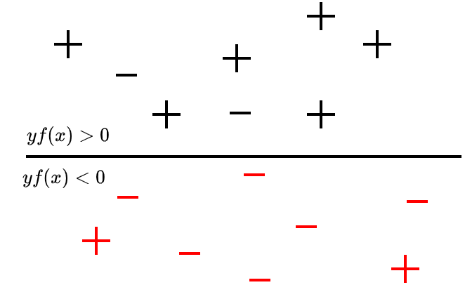
Here $Y$ is the output of our model. Basic mathematics tells that if the sign of $f(x)$ and y are different, the product will be negative and so it goes to negative side of the decision boundary. Hence all misclassified points are now on the negative side of the boundary. We assign a loss of 1 to the points on the lower side of the boundary to imply that misclassified points have to pay more penalty. The value can be any positive number in actual practice. There is zero or negligible loss to the points on the upper side of the boundary which are correctly classified points. For the points with $yf(x)>=1$, the hinge loss is zero and for points with $yf(x)<1$, the hinge loss increases tremendously and the upper bound of hinge loss, i.e. $1-yf(x)$ increases exponentially.
The mathematical formula for hinge loss in SVM is,
$L= max(0, 1-y^i (W ^T X+b))$
Here $L$ gives the loss at any instance and $X^i$ and $y^i$ represents $i^{th}$ instances in the training set and $b$ is the bias term
To be specific, $L = 0$ if $y^i (W ^T X+b>=0)$ and $1- y^i(W^ T X+b)$ otherwise. This formulation is called loss minimization condition.
Here $W$ is a vector of any length perpendicular to the hyperplane and $x$ is the vector corresponds to the point lies on any side of the hyperplane.
The equation of the hyperplane $H$ is, $W^TX+b = 0$
As $H^+$ and $H^-$ are at distance +1 and -1 respectively,
The equation for $H^+$ and $H^-$ are,
$H^+: W ^T X+b=+1$
$H^-: W^ T X+b=-1$
Worthmentioning here, the RHS of these equation need not be +1 or -1 always. The only requirement is the hyperplanes $H^+$ and $H^-$ should be at equivalent distance from the margin maximizing hyperplane $H$.
Also, $Y^i$ is the class label means $Y^i$ is positive for positively classified points and $Y^i$ is negative for negatively classified points.
$H^+$, $y^i(W ^T X+b)=+1$ ( as $Y^i$ is positive and $W^T X+b=+1$) and
$H^+$, $y^i(W^T X+b)=+1$ ( as $Y^i $is negative and $W^T X+b=-1$)
By applying simple mathematics, we can extract the value of margin, that is the distance between $H^+$ and $H^-$ as,
$D= \frac{2}{||W||}$
If $H^+$ and $H^-$ are not at unit distance and suppose at a distance of constant $C$ then $D= \frac{2C}{||W||}$
For simplicity of mathematics, we assume the positive and negative hyperplanes are at unit distance from H. Now we have to find out the $W^*$ and $b^*$ which maximizes the margin,
Mathematically,
$(W^*, b^* ) = argmax(w, b) [ \frac{2}{||W||}]$ or $argmin(a,b)\frac{||w||}{2}$ such that $y^i(W^TX+b)>=0$ for all points lie on either side of the hyperplane. This is the constraint optimization problem we have to solve while doing classification/regression using SVM.
The aforementioned optimization cannot be done for points identified as misclassified after we select the margin maximization hyperplane. Hence such an optimization condition is called hard margin SVM.
But we can modify this equation to some extent, if the point is at halfway between $H$ and $H^+$,
The equation becomes,
$y^i(W^T X+b)=+1-0.5=0.5$
If it is between H and $H^-$,
$y^i(W^T X+b)=+1-1.5=-0.5$ and so on
In general, $y^i(W^T X+b) =1-\epsilon$
Where $\epsilon$ is the distance of the misclassified point from the hyperplane in the incorrect direction.
Hence the generalized form of optimization problem becomes,
$(W^*, b^* ) = argmin(w,b) \frac{||w||}{2}+K \frac{1}{n}(\epsilon_i)$ such that $y^i(W^TX+b)>=1-\epsilon_i$ for all i and $\epsilon_i>=0$
Here, $K$ is the hyperparameter and $\frac{1}{n (\epsilon_i)}$ is the average distance of misclassified points from the hyperplane.
The term $\frac{1}{n(\epsilon_i)}$ is the hinge loss of the model which we want to minimize. This formulation of SVM is called soft margin SVM or the primal form SVM.
As the value of hyperparameter increases, $\frac{1}{n \epsilon_i}$ decreases in order to balance the overall weightage of the second term. Hence the tendency of the model to misclassify points reduces. But higher values of hyperparameter often led to
overfitting of the model.
In contrary if the value of hyperparameter is low, the first term is the equation which is the regularization term become more important and it led to overfitting the model.
The equation for soft margin SVM can be rewritten as,
| $\max_\alpha \sum_{i=1}^m\alpha_i -\frac{1}{2}\sum_{i=1}^m\sum_{j=1}^m\alpha_i\alpha_jy_iy_jx_i\cdot x_j \\ subject\space to\space \alpha_i \ge 0, i=1…m, \sum_{i=1}^m{a_iy_i}=0$ |
Here $K(x_i, x_j)$ are called kernal function. The equation is called kernel SVM. Whereas, the equation of SVM without replacement to kernel function are called linear SVM If we are given a query point $x_q$ , we can easily find the class label of it with the help of this kernel function such that, the class label of $X_q$, that is,
$f(x_q)=\sum_{i=1}^n\alpha_iy_iK(x_i,x_q)+b$
In situations when the data points belong to different classes are distributed as in fig. and difficult to separate with a hyperplane as, linear SVM fails. In such situations kernel SVM with correct kernel function can solve the problem.

Support vector machines kernel functions converts non separable problems to separable forms by transforming low dimensional input space to higher dimensional space. We can custom select the suitable kernel such as linear, polynomial, RBF(Radial Basis Function) or sigmoid for particular problem.
Unit vector normal to a plane w.r.t point of interest
The following code snippet creates and plots a 2D plane, a data point and the unit normal vector of the plane w.r.t to the data point.
import numpy as np
import matplotlib.pyplot as plt
from random import random, randint

INTERCEPT_START = -3
INTERCEPT_STOP = 3
XSTART = -3
XSTOP = 3
OFFSET = 1


def generateParams():
    m = random()-0.5
    C = randint(INTERCEPT_START, INTERCEPT_STOP)
    return m, C


def generateData(m, C):
    x = np.arange(XSTART, XSTOP)
    y = m*x+C
    p = randint(XSTART+OFFSET, XSTOP-OFFSET)
    q = randint(INTERCEPT_START+OFFSET, INTERCEPT_STOP-OFFSET)
    return x, y, p, q


def plotScene1(x, y, p, q):
    plt.plot(x, y, c='k', label='2d plane')
    plt.scatter(p, q, c='m', marker='*', label='data point')
    plt.ylim([INTERCEPT_START-OFFSET, INTERCEPT_STOP+OFFSET])
    plt.xlim([XSTART-OFFSET, XSTOP+OFFSET])
    plt.xlabel('x')
    plt.ylabel('y')


def plotScene2(w1, w0, x1, x0):
    svector = np.array([w1, w0])
    norm_vector = svector/np.linalg.norm(svector)
    plt.quiver(x1, x0, norm_vector[0], norm_vector[1], label='normal vector')
    plt.legend()
    plt.show()


if __name__ == '__main__':
    slope, intercept = generateParams()
    x, y, p, q = generateData(slope, intercept)
    plotScene1(x, y, p, q)
    plotScene2(1, -1/slope, p, q)

Conclusion
Support vector machines use hyperplanes or kernel functions to perform classification/regression of features based on the geometry of distribution of data points in space. To be concise, SVM is a supervised machine learning model works based on the geometrical properties of the features under consideration for the study.
Pingback: K-Nearest Neighbors Algorithm - Intuitive Tutorials
Pingback: Large Language Models in Deep Learning - Intuitive Tutorials