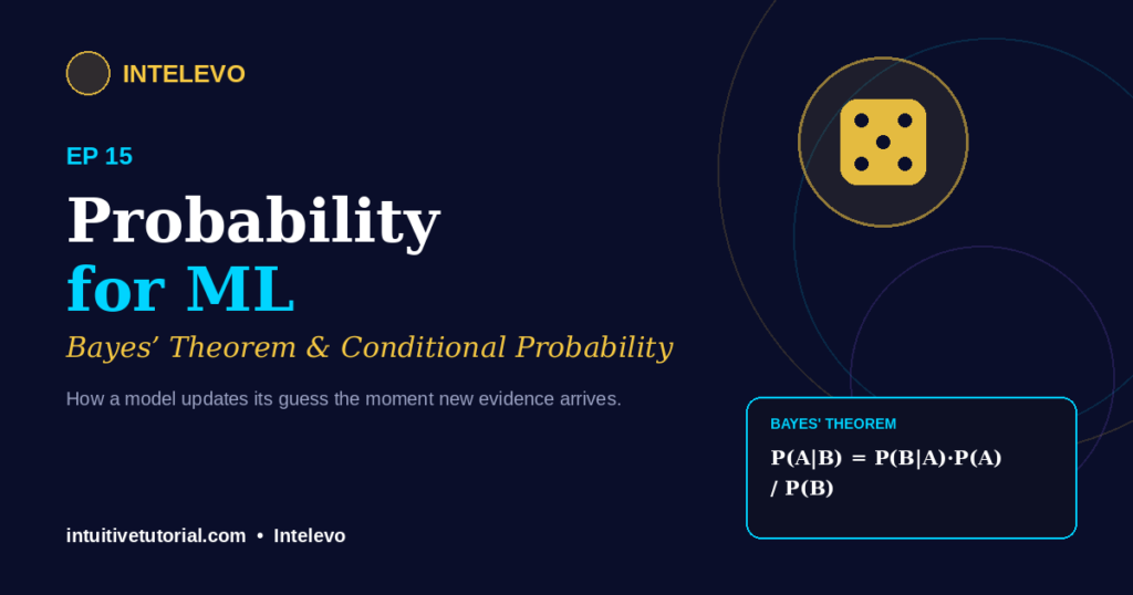
Every machine learning model makes a guess. Then, it gets new information. So, it updates that guess. This simple loop sits at the heart of probability for machine learning, and it explains why your spam filter, your medical test, and even your weather app all work the same way underneath.
This article walks through the ideas from Episode 15 of the Intelevo series. You can watch the full video breakdown on the Intelevo YouTube channel, where we build up each concept step by step, with live Python code. Here, we cover the same ground in writing, so you can read at your own pace and revisit the formulas whenever you need them.
Many learners feel intimidated the moment they see a probability formula. However, that fear usually comes from notation, not from the underlying idea. Once you strip away the symbols, probability turns out to be one of the most intuitive branches of mathematics you will ever encounter. You already use it every day, whether you check a weather app or decide if a deal sounds “too good to be true.”
By the end, you will understand probability, conditional probability, and Bayes’ theorem. Moreover, you will see exactly how these three ideas power real classifiers, from spam detection to disease screening. Let’s begin.
Why Probability Matters in Machine Learning
Uncertainty is everywhere. A model never knows anything for certain. Instead, it deals in likelihoods.
Consider a spam filter. It cannot know for sure whether a new email is spam. However, it can estimate how likely that email is to be spam, based on patterns it has seen before. That estimate is a probability.
The same logic applies far beyond email. A self-driving car cannot know with certainty whether a pedestrian will step onto the road. Instead, it constantly estimates the probability of that event, and it adjusts its speed accordingly. A search engine cannot know exactly which result you want. So, it ranks pages by the probability that each one satisfies your query. Even a medical diagnosis rarely comes as a flat “yes” or “no.” Instead, doctors and models alike work with likelihoods, then combine them with judgment.
Therefore, probability is not an optional extra in machine learning. It is the language models use to express confidence. Once you understand this language, model outputs stop feeling mysterious. Instead, they start making intuitive sense.
What Is Probability, Really?
Let’s strip away the jargon. Probability is just a fraction. You count how often something happens, and then you divide by everything that could happen.
Here is the formula:
P(A) = favorable outcomes / total outcomes
The result always falls between 0 and 1. A probability of 0 means the event never happens. A probability of 1 means it always happens. Everything else sits somewhere in between.
Let’s test this with a quick simulation. In Python, we can roll a die thousands of times and count how often we land on six:
import numpy as np

rolls = np.random.randint(1, 7, size=6000)

p_six = np.mean(rolls == 6)
print(p_six)
# → close to 0.167 (1 out of 6 faces)
As expected, the result lands close to 0.167, or roughly 1 in 6. This confirms the theory with real numbers, not just abstract reasoning.
Probability Powers Every Classifier
Now, let’s connect this to machine learning directly. Most classifiers do not simply output “yes” or “no.” Instead, under the hood, they compute a probability first. The yes/no label you see is just a rounded version of that number.
For example, scikit-learn models expose this directly through a method called predict_proba:
probs = model.predict_proba(email)
print(probs)
# → [0.13, 0.87]
# 13% not spam, 87% spam
Notice something important here. The model does not just say “spam.” It says “87% confident this is spam.” That distinction matters enormously in real-world systems, especially where a wrong guess carries a cost, such as medical diagnosis or fraud detection.
So, remember this: every classifier is secretly a probability engine wearing a yes/no costume. Once you see it this way, you will never look at a model’s output the same way again.
Conditional Probability: Updating Your Guess With New Information
Here is where things get more interesting. So far, we have only asked, “how likely is this event, on its own?” But real decisions rarely happen in isolation. Instead, we constantly update our guesses as new information arrives.
Think about weather forecasting. “What is the chance of rain today?” and “What is the chance of rain today, given that the sky just turned dark grey?” describe the exact same day. Yet, they produce very different answers, because the second question includes new evidence.
This is conditional probability, and its formula looks like this:
P(A | B) = P(A ∩ B) / P(B)
In plain English, this reads as “the probability of A, given that B has already happened.” Let’s see this in code, using our spam filter example:
import numpy as np

emails = np.array([1, 0, 1, 0, 1])
# 1 = contains "free"
is_spam = np.array([1, 0, 1, 0, 0])

# P(spam | contains "free")
mask = emails == 1
print(is_spam[mask].mean())
# → 1.0, far higher than the overall average
Here, we filter our data down to only the emails containing the word “free.” Then, we check what fraction of those specific emails turned out to be spam. The result jumps sharply higher than the overall spam rate, because we have narrowed our focus using relevant evidence.
Every Feature Narrows the Guess
A machine learning model rarely asks a single question. Instead, it asks many small conditional questions, one after another, and each new clue narrows the guess further.
Consider this progression:
p_spam = 0.50
p_spam_given_free = 0.90
p_spam_given_free_and_link = 0.97

print(p_spam, p_spam_given_free, p_spam_given_free_and_link)
# → 0.50 → 0.90 → 0.97
Notice how the probability climbs with each additional clue. Without any information, the model starts at a neutral 50%. Once it spots the word “free,” confidence jumps to 90%. Then, once it also spots a suspicious link, confidence climbs further, to 97%.
This is exactly how real models process features. Every column in your dataset acts as one more piece of conditioning evidence. As a result, before a model can make a confident decision, it needs to understand how each feature shifts the underlying odds.
Probability vs. Statistics: What Is the Difference?
At this point, you might wonder how probability connects to the statistics concepts from our previous episode. In Episode 14, we covered mean, variance, and distribution. Those three ideas describe data you already have. In contrast, probability describes data you have not seen yet.
Here is a simple way to remember the distinction. Statistics looks backward. It summarizes what already happened in your dataset. Probability looks forward. It estimates what is likely to happen next.
In practice, machine learning constantly moves between the two. First, a model studies historical data using statistics. Then, it uses probability to make predictions about new, unseen examples. So, these two branches of math work as partners, not competitors. Each one supports the other at a different stage of the pipeline.
Bayes’ Theorem: Flipping the Question Around
Now we reach the centerpiece of this episode: Bayes’ theorem. This idea sounds intimidating at first, but it solves a very ordinary problem.
Often, you know one direction of a relationship, but you actually need the other. For instance, you might know how often the word “free” appears in spam emails. However, what you actually want to know is the reverse: given that this specific email contains the word “free,” how likely is it to be spam?
Bayes’ theorem exists precisely to flip this question around. Here is the formula:
P(A | B) = P(B | A) · P(A) / P(B)
Think of it like detective work. You start with a hunch. Then, you spot a clue. Finally, you revise your suspicion based on that clue. Bayes’ theorem is simply that revision process, written as arithmetic.
A Worked Example: Spam Filter Math
Let’s put real numbers into the formula, so the idea sticks. Suppose 20% of all email is spam. That is our starting belief, before we look at any specific message.
Next, suppose we know two additional facts from past data:
- The word “free” appears in 60% of spam emails.
- The word “free” appears in only 5% of normal emails.
Now, a new email arrives, and it contains the word “free.” How should we update our belief? Let’s compute this directly in Python:
p_spam, p_not_spam = 0.20, 0.80
p_free_given_spam = 0.60
p_free_given_not_spam = 0.05

top = p_free_given_spam * p_spam
bottom = top + (p_free_given_not_spam * p_not_spam)
print(top / bottom)
# → belief jumps from 20% to about 75%
The result is striking. Our belief jumps from a modest 20% all the way up to roughly 75%, purely because of one word. This single calculation captures the entire spirit of Bayesian updating: start with a belief, observe evidence, then revise.
Building a Tiny Naive Bayes Classifier in Python
Let’s now combine everything into one small, working classifier. We will use scikit-learn’s Gaussian Naive Bayes model, which applies Bayes’ theorem automatically across every feature in your dataset.
from sklearn.naive_bayes import GaussianNB

# words → simple numeric signal
X = [[1], [0], [1], [0], [1]] # "free"?
y = [1, 0, 1, 0, 0] # spam?

model = GaussianNB()
model.fit(X, y)

print(model.predict_proba([[1]]))
# → probability this new email is spam, given it has "free"
Why do we call this approach “naive”? Because it assumes each clue affects the odds independently of every other clue. In reality, this assumption rarely holds perfectly. Words in an email often correlate with each other. Nevertheless, this simplification works remarkably well in practice, and it remains fast, interpretable, and easy to train, even on huge datasets.
Where This Math Hides in Everyday Life
At this point, you might think Bayes’ theorem sounds like specialized, academic math. However, it quietly runs behind decisions you already trust every single day.
Spam filters. Every time your inbox correctly labels junk mail, a Bayesian update just happened in milliseconds.
Medical tests. A positive result updates the probability of illness. Importantly, it rarely means “you are certainly sick.” Instead, it means your probability of being sick has increased, based on the test’s accuracy and how rare the condition actually is.
Weather forecasts. That “70% chance of rain” figure comes directly from how often similar past days led to rain. Meteorologists essentially run a large-scale conditional probability calculation.
Recommendation systems. Streaming platforms constantly update their guess about what you will watch next, based on what you have already watched. Each click you make becomes new evidence for their internal model.
Once you notice this pattern, you will start spotting it everywhere. Uncertainty, evidence, and updated belief form a loop that appears across nearly every intelligent system.
Quick Recap: The Three Building Blocks
Let’s tie everything together with a short summary.
First, probability tells you how likely a single outcome is, expressed as a simple fraction between 0 and 1.
Next, conditional probability tells you how new evidence changes that likelihood. It narrows your focus to a more relevant group before recalculating the odds.
Finally, Bayes’ theorem flips the condition around. It lets you move from what you already know to what you actually want to know, using one clean formula.
Together, these three ideas form the mathematical backbone behind spam filters, diagnostic tools, recommendation engines, and countless other systems you interact with daily.
Frequently Asked Questions
Is Bayes’ theorem hard to learn? No, not really. The formula looks dense at first glance. However, the underlying idea stays simple: start with a belief, observe evidence, then revise. Once you practice with a few worked examples, like the spam filter above, the formula stops feeling abstract.
Why is Naive Bayes called “naive”? It assumes every feature affects the outcome independently of every other feature. In real datasets, this assumption rarely holds perfectly, since features often correlate with each other. Even so, this simplification keeps the model fast and interpretable, and it still performs remarkably well across many real-world tasks.
Do I need calculus to understand probability? No, you do not. Probability for machine learning relies mainly on arithmetic: fractions, multiplication, and division. Calculus becomes essential later, once you study how models learn through gradient-based optimization. We cover that topic next, in Episode 16.
Where does probability show up beyond classification? Almost everywhere. Recommendation engines, ranking algorithms, anomaly detection systems, and even generative AI models all rely on probability distributions to make decisions under uncertainty. Once you understand the basics, you will recognize this pattern across nearly every corner of machine learning.
What’s Next: Calculus for Machine Learning
Probability explains how a model reasons under uncertainty. However, it does not explain how a model learns from its mistakes. That story belongs to calculus.
In Episode 16, we will explore derivatives, gradients, and the chain rule, using the same simple, intuitive approach. You will discover exactly how a model knows which direction to adjust itself, one small slope at a time, without drowning in dense notation.
Watch the Full Video Breakdown
This article covers the core ideas from Episode 15 of the Intelevo YouTube series, but the full video walks through every example live, with on-screen code and visual explanations. If reading sparked your curiosity, watching the video will deepen it further.
While you are there, consider subscribing to the channel. New episodes continue building this machine learning roadmap, one intuitive idea at a time. And if this article helped clarify probability for machine learning, share it with someone who is currently staring at a textbook full of intimidating formulas. Sometimes, all a concept needs is a simpler story.