Every machine learning model learns the same way. It guesses, checks how wrong it is, and adjusts. Then it repeats that cycle thousands of times. Underneath that entire process sits one subject: calculus.
This might sound intimidating. However, calculus for machine learning doesn’t need textbook formulas or years of math class. It needs one picture and three ideas. In this article, we’ll build that picture together, then connect each idea to real Python code. This is EP16 of the Intelevo Machine Learning series, and it also accompanies our YouTube video on the same topic. Watch the video for the full walkthrough, and use this article as your written reference and notes.
By the end, you’ll understand derivatives, gradients, and the chain rule well enough to explain them to a friend. No dense notation required. Whether you’re new to machine learning or brushing up before a deep learning course, this breakdown gives you the intuition first. The formulas come easier once the picture is clear.
Why Calculus Matters in Machine Learning
Picture this. You’re standing in thick fog on a hillside, and you want to reach the lowest point in the valley. You can’t see the bottom. But you can feel which way the ground slopes under your feet. So you take a step in that direction, and you check again.
That feeling is calculus. You already understand it. You just haven’t called it that before.
A machine learning model does the exact same thing. It starts with a random guess. Then it measures its error, called the “loss.” Next, it feels which direction reduces that error, and it nudges itself that way. It repeats this process again and again until the error gets as small as possible.
Three ideas make this possible:
- The derivative answers “how fast is something changing?”
- The gradient answers “which direction should I move?”
- The chain rule answers “how do changes ripple through connected steps?”
Keep this hillside picture in your mind. We’ll return to it throughout this article.
The Derivative: Your Model’s Speedometer
A derivative is just a slope. It tells you how much an output changes when you nudge an input by a tiny amount. That’s the entire idea, expressed as a single number.
Consider a simple function, f(x) = x². At the point x = 3, how steep is this curve? We can estimate it in Python without any calculus textbook:
def f(x):
    return x ** 2

x, h = 3, 0.0001
slope = (f(x + h) - f(x)) / h
print(slope)
# -> 6.0
This code nudges x by a tiny amount, h, and measures how much the output moves. The result, 6.0, is the slope of the curve at that exact point. This is the derivative.
Two things are worth remembering here. First, a derivative is just “rise over run” — for a small step in x, how much does the output move? Second, a slope of zero means you’re standing on a peak, a valley, or a flat stretch. There’s nowhere to go from there, which is exactly the point where training stops improving.
Think of the derivative as your model’s speedometer. It tells the model how fast its error is changing right now, at this exact moment.
Derivatives Show Up Everywhere in ML
Training a model means constantly asking one question: if I nudge this weight slightly, does my error get better or worse? That question is a derivative, and a model asks it millions of times during training.
Here’s a small example. Suppose our loss function depends on a weight, w:
loss = lambda w: (w - 4) ** 2

w, h = 1.0, 0.0001
grad = (loss(w + h) - loss(w)) / h
print(grad)
# -> -6.0
The result is negative six. That negative sign matters a lot. It tells us that increasing w will reduce the loss. Without this information, the model would have no idea which direction to move.
So, every “trained” model got that way by asking millions of these tiny “which way?” questions. A derivative answers each one. If a model can’t measure its own slope, it simply cannot know which way to move.
The Gradient: A Compass for Many Weights
Real models rarely have just one input. Instead, they have hundreds, thousands, or even billions of weights. A gradient extends the idea of a derivative to all of them at once. It calculates the slope for every single weight, simultaneously, and packages the result into one arrow.
def loss(w1, w2):
    return w1**2 + w2**2

w1, w2 = 3.0, -2.0
grad_w1, grad_w2 = 2 * w1, 2 * w2
print(grad_w1, grad_w2)
# -> tells us how to nudge BOTH weights at once
Think of a gradient as a compass needle. It always points toward the steepest climb. Therefore, to go downhill fastest, you simply walk in the exact opposite direction the compass points. This one flip — moving opposite the gradient — is the foundation of how every model learns.
Gradient Descent: Walking Downhill on Purpose
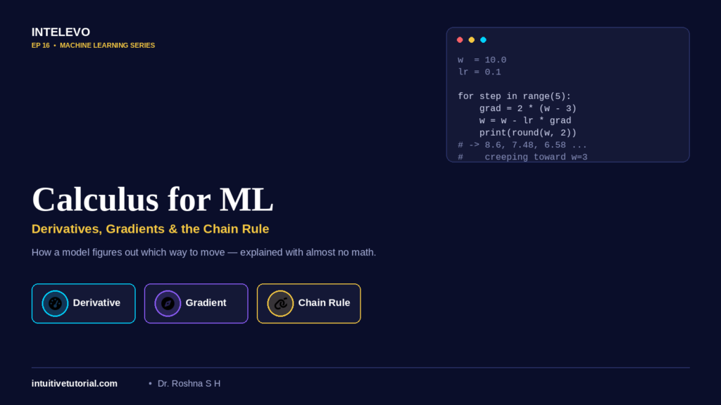
Now we can put the gradient to work. Take a small step opposite the gradient. Then check the slope again. Repeat. That loop is literally how every machine learning model learns, and it has a name: gradient descent.
w  = 10.0        # random start
lr = 0.1         # step size

for step in range(5):
    grad = 2 * (w - 3)  # slope
    w = w - lr * grad   # step downhill
    print(round(w, 2))
# -> 8.6, 7.48, 6.58, 5.87, 5.29
#    creeping toward w = 3
Watch the numbers. They creep closer and closer to 3, which happens to be the lowest point of this particular loss function. This tiny loop, repeated thousands of times, is the entire training step inside every neural network you’ve ever used.
In one sentence: gradient descent means feel the slope, take a small step down, and repeat until flat.
The Chain Rule: Connecting the Dots
So far, we’ve dealt with simple, one-step functions. However, real models stack functions on top of each other, layer after layer. The chain rule tells us exactly how a change at the very first layer ripples all the way through to the final output.
Suppose y depends on u, and u depends on x:
def u(x): return x + 1
def y(u_val): return u_val ** 2

dy_du = 2 * u(3)   # outer slope
du_dx = 1          # inner slope
print(dy_du * du_dx)
# -> 8, the combined slope
To connect these two slopes, we simply multiply them together. That’s the entire chain rule. Picture a row of dominoes. Push the first domino, x, and the chain rule tells you exactly how hard the very last domino, y, gets hit.
Backpropagation: The Chain Rule at Scale
A neural network can have dozens, or even hundreds, of stacked layers. You’ve probably heard the word “backpropagation” before. In reality, it’s nothing more than the chain rule, applied layer by layer, walking backward from the error all the way to every individual weight.
layer1 = lambda x: x * 2   # w1 = 2
layer2 = lambda h: h + 5   # bias

x = 3
h = layer1(x)      # forward pass
out = layer2(h)

d_out_d_h, d_h_d_x = 1, 2
print(d_out_d_h * d_h_d_x)  # 2
Think of it as a relay race. Every layer hands its slope backward to the layer before it. That relay race, repeated across every layer in the network, is exactly what backpropagation means. Consequently, every “AI learns” headline you read is quietly this exact multiplication, happening millions of times per second.
Putting It All Together: The Training Loop
Derivative, gradient, and chain rule. Chained together, they become the training loop that sits behind every deep learning model, and it only takes a few lines of code:
import numpy as np

w  = np.array([5.0, -2.0])
lr = 0.1

for epoch in range(3):
    grad = 2 * w        # derivative, for every weight
    w = w - lr * grad   # gradient descent step
    print(w)
# -> weights creep toward zero, the lowest-loss point
Frameworks like PyTorch and TensorFlow do exactly this, except the chain rule gets computed automatically, across millions of weights. This process even has a name: autograd. This five-line loop, scaled up dramatically, is genuinely how today’s largest AI models learn.
Derivative vs. Gradient vs. Chain Rule, at a Glance
| Concept | What It Is | Analogy | In One Line |
|---|---|---|---|
| Derivative | How fast one thing changes | A speedometer reading | dy / dx |
| Gradient | The slope for every input, at once | A compass pointing uphill | ∇f |
| Chain Rule | How slopes combine across steps | A row of dominoes | dy/dx = dy/du · du/dx |
This table sums up everything we’ve covered. Whenever you get confused, come back to this comparison.
Test Yourself: Quick Gut Check
Here’s a scenario. A model’s loss has a slope of −4 at its current weight. The learning rate is 0.1. Which way, and by how much, should the weight move?
Take a moment before reading further.
The answer: increase the weight by 0.4, opposite the slope. Here’s why. A negative slope means increasing the weight lowers the loss. The formula confirms this — negative learning rate times gradient equals −0.1 × (−4), which equals +0.4.
If you got this right, calculus for machine learning is officially clicking for you.
You Already Use This Math Every Day
Here’s something encouraging. You’ve been using these three ideas your entire life, just not by these names.
Cruise control in your car feels the road’s slope and adjusts the throttle. That’s a derivative at work. GPS rerouting recalculates the fastest direction the instant the road changes. That’s a live gradient. Your thermostat nudges the heater a little, checks the result, and nudges again. That’s gradient descent, quietly running inside your wall. Finally, your fitness tracker chains together your pace, incline, and heart rate to estimate your real effort. That’s the chain rule at work.
So, derivatives, gradients, and the chain rule aren’t locked away inside a math classroom. They’re quietly steering things you interact with every single day.
Common Pitfalls to Watch For
Understanding the theory is one thing. Applying it correctly is another. So, here are three pitfalls that trip up beginners working with calculus for machine learning.
First, a learning rate that’s too large causes the model to overshoot the valley entirely. Instead of settling near the lowest point, the weights bounce around wildly, and the loss might even increase. Second, a learning rate that’s too small makes training painfully slow. The model inches toward the answer, and you might quit before it gets there. Therefore, most practitioners start with a moderate rate and adjust based on how the loss behaves.
Third, watch out for vanishing gradients in deep networks. Remember, the chain rule multiplies slopes together across many layers. If those slopes are small fractions, multiplying dozens of them together produces a number close to zero. As a result, early layers barely update at all. Modern architectures use specific tricks, like different activation functions and normalization layers, to fight this exact problem. You don’t need to memorize the fixes right now. Just remember that this is why the chain rule matters beyond a single homework problem — it explains real design decisions inside modern AI systems.
Recap: What We Covered
Let’s tie everything together. We learned three building blocks: the derivative, the gradient, and the chain rule. You have seen how a model feels its own slope and steps downhill, one tiny nudge at a time. We watched simple Python code turn each idea into a working training loop. We also looked at common pitfalls, like learning rates that are too large or too small, and why vanishing gradients matter in deep networks. Finally, we connected the chain rule to backpropagation, the real engine running behind every deep neural network.
None of this required heavy notation. It only required one picture: fog on a hillside, and the feeling of finding your way down. Next time someone mentions gradients or backpropagation, you’ll have a concrete image in mind instead of a wall of symbols.
What’s Next
In EP17, we move to NumPy for machine learning. We’ll cover arrays, broadcasting, and vectorized operations. Most importantly, we’ll see how to run all of this math across millions of numbers at once, without writing a single loop.
If this article helped the concepts click, the companion YouTube video walks through every example step by step, with visuals for each analogy. Watch it, then come back here anytime you need a quick written refresher.
You now understand calculus for machine learning well enough to follow any training loop you encounter. That’s a real milestone. Keep going.
This article accompanies Episode 16 of the Intelevo Machine Learning series on YouTube. Subscribe to Intelevo for the full series, and check intuitivetutorial.com for written notes on every episode.