Bag of Words counts your words. TF-IDF weighs them. But neither one understands them. Ask either method whether “cat” and “kitten” are related, and you get silence. Both words are just columns in a spreadsheet, as far apart as “cat” and “airplane.”
That gap is exactly what word embeddings close. In this article, we walk through what word embeddings are, how Word2Vec and GloVe learn them, and how you can start using them today with a few lines of Python. This is the companion write-up to Episode 94 of the Intelevo YouTube series, so if you prefer to watch and follow along, the video covers the same ground with visuals and live code.
By the end, you’ll see why “king minus man plus woman” lands you on “queen,” and why that’s not a party trick. It’s the whole point.
The Problem With Just Counting Words
Let’s start with where we left off. In Episode 93, we converted cleaned sentences into numbers using two techniques: Bag of Words and TF-IDF. Bag of Words counts how many times each word appears. TF-IDF goes a step further and boosts rare, meaningful words while muting common ones like “the” or “is.”
Both techniques work well for many tasks. However, they share a blind spot. Neither one encodes meaning. To a Bag of Words vector, every word is just a slot in a giant list. “Cat” and “kitten” get separate columns, with zero connection between them. So do “happy” and “joyful.” The model has no way to know these words are related.
This matters because language is full of synonyms, near-synonyms, and related concepts. A sentiment classifier trained only on raw word counts might miss that “fantastic” and “amazing” mean almost the same thing. As a result, it needs to see both words in training data separately, rather than generalizing from one to the other.
So here’s the question this article answers: what if a computer could tell that “cat” and “kitten” are practically the same idea, without anyone teaching it a single grammar rule? That’s exactly what word embeddings do.
A Map Made of Meaning
Before the formulas, let’s build intuition with an analogy. Think about a real map. Cities that sit close together usually share a similar climate and culture. Paris and Brussels, for instance, are near each other and share plenty in common. Paris and Tokyo do not.
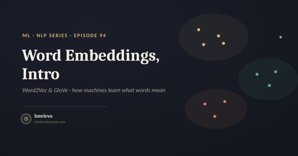
Now imagine a similar map, but built for words instead of cities. Instead of geography, this map uses meaning. Words that show up in similar sentences end up parked near each other. “Cat,” “kitten,” “dog,” and “puppy” cluster in one neighborhood. “Car,” “bus,” and “train” form their own cluster elsewhere. A word like “airplane,” used in very different contexts, sits far from all of them.
That’s the entire idea behind word embeddings. Meaning becomes location. Once words have positions, you can measure distance, and distance becomes a proxy for similarity. This single shift makes an enormous difference in how machines process language.
What Are Word Embeddings, Exactly?
Now let’s put a precise definition on this idea. A word embedding represents each word as a list of numbers, called a vector. The numbers aren’t arbitrary. They’re positioned so that words used in similar ways end up close together in that numeric space.
Three things are worth remembering here.
First, every word becomes a vector. Typically, that vector holds somewhere between 50 and 300 numbers, though larger models can use more. Second, distance between two vectors mirrors similarity in meaning. Words that behave alike in sentences end up with similar numbers. Third, nobody writes these numbers by hand. A model discovers them automatically by scanning huge amounts of text.
This last point matters. Unlike a hand-built thesaurus, these vectors need no manual curation. Feed a model enough text, and the relationships emerge on their own.
You Are the Company You Keep
So how does a model figure out which words belong near each other? The answer comes from linguistics, and it’s called the distributional hypothesis. The idea is simple: words that tend to appear near the same neighboring words usually share a similar meaning.
Consider three words: “coffee,” “tea,” and “rocket.” Look at what tends to appear around each one.
| Word | cup | drink | morning | engine | launch |
|---|---|---|---|---|---|
| coffee | yes | yes | yes | no | no |
| tea | yes | yes | yes | no | no |
| rocket | no | no | no | yes | yes |
“Coffee” and “tea” share nearly every context word. As a result, they land close together on the map. “Rocket” shares none of those words, so it lands far away, closer to words like “engine” and “launch” instead.
This pattern, repeated across millions of sentences, is the mechanism these vectors actually exploit. No dictionary definitions get involved. Context alone does the work.
Building a Tiny Word2Vec Model in Python
Let’s move from theory to code. Word2Vec, one of the earliest and most influential embedding methods, learns vectors directly from raw sentences. Here’s a minimal example using the gensim library.
from gensim.models import Word2Vec

sentences = [
    ["cat", "sat", "on", "the", "mat"],
    ["dog", "sat", "on", "the", "rug"],
    ["kitten", "played", "near", "the", "mat"]
]

model = Word2Vec(sentences, vector_size=50, window=2, min_count=1)

print(model.wv["cat"][:5])
# [ 0.012  -0.045   0.078   0.031  -0.009 ]

print(model.wv.most_similar("cat"))
# [('kitten', 0.91), ('dog', 0.84), ('mat', 0.62)]
First, we import Word2Vec and define a tiny list of sentences. Next, we create the model in a single line. The vector_size parameter sets how many numbers represent each word, here 50. The window parameter controls how many neighboring words the model considers on each side, and min_count=1 keeps even rare words instead of dropping them.
After training, model.wv gives you the vector for any word. We print the first five of fifty numbers for “cat” just to see real output. Then, most_similar() shows which words land closest to “cat” on the map. Even with only three tiny sentences, the model correctly groups “cat” near “kitten” and “dog.” Feed it millions of real sentences instead of three toy ones, and this same mechanism produces genuinely useful vectors.
How Word2Vec Actually Learns
Under the hood, Word2Vec never sees a dictionary or a grammar rule. Instead, it plays one of two guessing games, repeated millions of times.
The first version is called CBOW, short for Continuous Bag of Words. Given the neighboring words, like “the ___ sat,” the model has to guess the missing word in the middle. In this case, the correct answer is “cat.”
The second version is called Skip-gram, and it flips the game around. Given one word, like “cat,” the model has to guess which words are likely to sit around it, such as “sat” or “mat.”
Either way, the mechanism stays the same. Right or wrong, the model nudges each word’s numbers a small amount after every guess. Because this process repeats across millions of sentences, words that keep showing up in similar spots gradually settle near each other. Over time, a coherent map of meaning emerges from nothing more than repeated prediction and correction.
GloVe: Counting Coincidences Across an Entire Library
Word2Vec isn’t the only path to good word vectors. GloVe, short for Global Vectors for Word Representation, takes a different approach entirely.
Here’s an analogy to make the difference clear. Word2Vec behaves like a student reading one sentence at a time, guessing as it goes. GloVe behaves more like a librarian who first reads every book in the library, tallies how often each pair of words appears together across the whole collection, and only then builds the map from those totals.
Concretely, GloVe constructs one large table recording how often word A appears near word B, anywhere across the entire corpus. Then, it fits each word’s vector so that the relationships between vectors match those global counts as closely as possible.
The key difference comes down to scope. Word2Vec learns from small, local windows, sentence by sentence. GloVe learns from global statistics, tallied once across everything. Both techniques produce a useful map of meaning, but they arrive there through different routes.
Measuring Closeness: Cosine Similarity
Once you have these vectors, you need a way to measure how close two of them actually are. The standard tool for this is cosine similarity.
similarity(A, B) = (A · B) / (|A| × |B|)
Don’t worry about calculating this by hand. Libraries like gensim compute it instantly with a single function call. What matters is what the resulting number means. A score of 1.0 means the two vectors point in exactly the same direction, indicating very similar words. Whereas, a score of 0 means the words are unrelated. A score of −1 means they point in opposite directions.
In plain terms, the dot product in the numerator measures how much two vectors point the same way. The magnitudes in the denominator normalize that score, so the comparison stays fair regardless of how “long” any particular word’s vector happens to be. Together, these two pieces turn a list of raw numbers into a meaningful similarity score.
Vector Arithmetic: King − Man + Woman = Queen
Here’s where word embeddings become genuinely impressive. Because embeddings capture relationships as directions in space, you can add and subtract word vectors like ordinary numbers, and land on another real word.
| Start Word | Operation | Nearest Result | What It Shows |
|---|---|---|---|
| King | − Man + Woman | ≈ Queen | Gender direction |
| Paris | − France + Italy | ≈ Rome | Capital-of direction |
| Walking | − Walk + Swim | ≈ Swimming | Tense direction |
Take “King,” subtract “Man,” add “Woman.” The closest resulting vector lands on “Queen.” Take “Paris,” subtract “France,” add “Italy.” You land near “Rome.” Take “Walking,” subtract “Walk,” add “Swim.” You land near “Swimming.”
Nobody taught the model a rule about kings, queens, or capital cities. Instead, this pattern falls directly out of each word’s position in the vector space. Relationships like gender, geography, and grammatical tense get encoded as consistent directions, and arithmetic on those directions produces genuinely sensible results.
Using Pretrained Vectors in Python
In practice, you’ll rarely train word embeddings from scratch. Instead, you’ll load a pretrained model and start using it right away.
import gensim.downloader as api

wv = api.load("glove-wiki-gigaword-50")   # pretrained GloVe vectors

print(wv.similarity("cat", "kitten"))
# 0.73   -> close in meaning

result = wv.most_similar(positive=["king", "woman"], negative=["man"])
print(result[0])
# ('queen', 0.85)
First, we import gensim’s downloader module and load a GloVe model pretrained on Wikipedia text. Next, wv.similarity() confirms that “cat” and “kitten” score high, at 0.73, meaning they’re close together in the vector space. Finally, most_similar() lets us test the king-minus-man-plus-woman example ourselves. Positive words get added, negative words get subtracted, and the top result comes back as “queen,” with a similarity score of 0.85.
Notice the pattern here. It mirrors the same fit_transform-style simplicity you already used with CountVectorizer and TfidfVectorizer back in Episode 93. Swap in a pretrained model, and analogies like this one become a single line of code.
Word2Vec vs. GloVe: Which One Should You Use?
At this point, a natural question comes up. Should you use Word2Vec or GloVe? The honest answer is that it depends on your data and your goals.
| Word2Vec | GloVe | |
|---|---|---|
| What it learns from | Small sliding context windows | Whole-corpus co-occurrence counts |
| Training style | Predicts words, like a guessing game | Fits vectors to match global counts |
| Captures best | Strong local patterns | Strong global statistics |
| Great for | Custom, domain-specific text | General-purpose pretrained vectors |
If you’re working with a specialized vocabulary, such as medical notes or legal contracts, training your own Word2Vec model on that specific text often works well. On the other hand, if you need general-purpose vectors quickly, a pretrained GloVe model, trained on massive general text, gets you up and running immediately. In many real projects, teams simply start with pretrained GloVe vectors and only train custom Word2Vec models if the domain proves specialized enough to need it.
Where Word Embeddings Fit In Your NLP Pipeline
Let’s zoom out and connect this to the bigger picture. A typical text pipeline looks like this.
First, you tokenize and clean a raw sentence, splitting it into words and normalizing case. Next, as covered in Episode 93, you can count those words with Bag of Words or weight them with TF-IDF. Today, we added a new stage: word embeddings, where words get vectors that actually capture meaning instead of just frequency. Finally, the result, whichever technique you choose, is a numeric vector ready to feed into a machine learning model.
Each stage builds on the one before it. Clean words become counted words. Counted words become weighted scores. And now, thanks to word embeddings, weighted vocabulary can become a genuinely meaning-aware vector. That upgrade matters enormously for anything involving similarity, clustering, or downstream classification.
Key Takeaways
Before wrapping up, here are three things worth remembering.
First, word embeddings place words on a map of meaning. Similar words automatically end up near each other, with no dictionary required. Second, Word2Vec guesses while GloVe counts. They’re two different roads leading to the same kind of map. Third, you’ll rarely train embeddings from scratch in practice. A library like gensim, combined with a pretrained GloVe or Word2Vec file, gets you a working map of meaning in just two lines of code.
Watch the Full Video
This article summarizes Episode 94 of the Intelevo YouTube series, but the video walks through every example with visuals, live code, and a full explanation of the map analogy. If you learn better by watching, check out the episode and follow along with the code yourself.
Coming up next, Episode 95 puts these word embeddings to work by building a full sentiment analysis model with classical machine learning. If today’s article helped things click, subscribe to Intelevo on YouTube so you don’t miss it, and drop a comment letting us know which part of word embeddings surprised you the most.