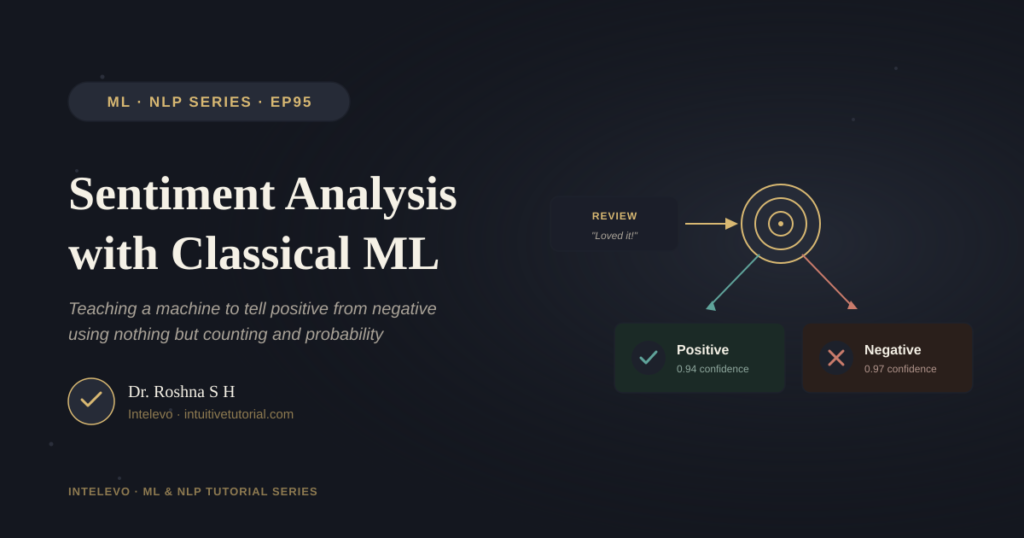
Every day, people leave millions of reviews online. Some praise a product. Others complain about it. Reading all of them by hand is impossible. So, how does a machine sort the good from the bad? That’s exactly what Sentiment Analysis with Classical ML solves. It teaches a computer to label text as positive or negative, without ever “feeling” a single word.
In this article, we’ll build that skill from scratch. First, we’ll clean messy text. Next, we’ll turn it into numbers. Then, we’ll let a classic machine learning model make the final call. Along the way, you’ll see real Python code, a friendly analogy, and the traps that catch beginners off guard. By the end, you’ll understand exactly how Sentiment Analysis with Classical ML works, and why it still powers so many real-world products today.
This post is the companion piece to Episode 95 of the Intelevo YouTube series. If you’d rather watch the full walkthrough, the video covers every step visually. But if you prefer reading at your own pace, keep going.
What Is Sentiment Analysis, Really?
Let’s start simple. Sentiment analysis means using a trained model to label a piece of text as positive, negative, or sometimes neutral. The model bases its decision purely on word patterns. It never actually understands feelings. Instead, it spots statistical clues that tend to show up in happy or angry writing.
Three ideas define this process. First, text goes in, and a label comes out. Second, the model learns from thousands of examples that humans already labeled by hand. Third, the model reacts to patterns, not emotions. It has no idea what “joy” feels like. However, it knows that the word “amazing” shows up far more often in five-star reviews than in one-star complaints.
So, why does this matter? Because Sentiment Analysis with Classical ML lets businesses process feedback at scale. A company can scan ten thousand reviews in seconds. Meanwhile, a human reader would need days.
The Big Analogy: Sorting Reviews by Ear
Here’s a mental picture worth keeping. Imagine a fast reader standing beside a conveyor belt. Reviews flow past her, one after another. She doesn’t read every sentence carefully. Instead, she listens for loaded words like “amazing” or “terrible.” Then, she tosses each review onto a matching pile.
This is almost exactly what a classical ML sentiment model does. It scans thousands of weighted words. Then, it sorts each review into a “positive” or “negative” bin. Unlike a human, though, it never gets tired. It never loses focus after review number four thousand. That consistency is the real superpower behind Sentiment Analysis with Classical ML.
Step One: Cleaning the Text
Before any counting begins, raw text needs a cleanup. Why? Because capital letters, punctuation, and filler words add noise. They carry no real opinion. So, a short preprocessing pipeline tidies everything first.
This pipeline typically includes five stages:
- Lowercase everything. “Amazing” and “amazing” should count as the same word.
- Strip punctuation. Exclamation marks and periods add clutter, not meaning.
- Remove stopwords. Words like “the,” “and,” and “is” appear everywhere. They rarely signal sentiment.
- Tokenize the text. This step splits a sentence into individual words.
- Stem or lemmatize. This step reduces words to their root form, so “disappointing” becomes “disappoint.”
Consider this example. The raw sentence reads: “The Service was SLOW… and honestly, quite disappointing!!” After cleaning, it becomes a tidy list: ["service", "slow", "honestly", "quit", "disappoint"]. That list is what the model actually sees. Nothing more, nothing less.
Step Two: Turning Words into Numbers
Classical ML models can’t read words directly. They only understand numbers. So, the next step converts clean text into a numeric format. For this task, TF-IDF remains the go-to method.
TF-IDF stands for “term frequency, inverse document frequency.” In simple terms, it scores each word based on how much it stands out. A rare, opinion-heavy word gets a high score. A common, everywhere word gets a low score.
Take a look at this example:
| Word | Count in Review | TF-IDF Weight | Why |
|---|---|---|---|
| “amazing” | 1 | 0.71 | Rare, opinion-heavy word |
| “the” | 3 | 0.02 | Appears everywhere, so it barely counts |
| “terrible” | 1 | 0.68 | Rare, strongly negative word |
Notice the pattern. “The” shows up three times, yet it scores almost nothing. Meanwhile, “amazing” appears just once, but it scores high. This weighting helps the model focus on words that actually carry sentiment.
Interestingly, word embeddings can also work here. You could average embedding vectors across an entire review. However, TF-IDF stays simpler and remains the more common choice for classical models. So, for this project, we’ll stick with it.
Step Three: Meet the Classifiers
Once every review becomes a row of numbers, a classifier can learn to split them. Three algorithms dominate this space:
- Naive Bayes weighs word evidence using probability. It’s fast, simple, and surprisingly strong on text data.
- Logistic Regression learns one weight per word. Then, it sums those weights and squashes the total into a probability.
- Linear SVM draws the widest possible boundary line between positive and negative reviews.
Each option has strengths. However, Naive Bayes offers the clearest starting point for beginners. Therefore, we’ll use it for today’s hands-on demo.
Naive Bayes: A Jury Counting Votes
Let’s build intuition before jumping into code. Picture every word in a review as a juror. During training, each juror learns how often it appeared in positive reviews versus negative ones. Then, at prediction time, every juror casts a vote. Whichever verdict receives the loudest combined vote wins.
The word “naive” simply means the jurors vote independently. They never confer with each other. This assumption isn’t perfectly realistic, but it works remarkably well in practice.
Here’s the one formula worth remembering:
P(positive | review) ∝ P(positive) × P(word₁ | positive) × P(word₂ | positive) × ...
Don’t worry about memorizing this. You’ll never compute it by hand. Instead, scikit-learn’s MultinomialNB() handles the math instantly. Still, understanding the logic helps demystify what’s happening under the hood.
Hands-On Python: Build a Sentiment Classifier
Now, let’s turn theory into code. The following example builds a working sentiment classifier in just a few lines.
from sklearn.feature_extraction.text import TfidfVectorizer
from sklearn.naive_bayes import MultinomialNB

vectorizer = TfidfVectorizer(stop_words="english")
X_train = vectorizer.fit_transform(reviews)   # text → TF-IDF numbers

model = MultinomialNB()
model.fit(X_train, labels)                    # labels: "pos" / "neg"

new_review = vectorizer.transform(["Absolutely loved this place!"])
print(model.predict(new_review))
# ['pos']
Let’s break this down step by step. First, we import TfidfVectorizer and MultinomialNB from scikit-learn. Next, we create a vectorizer and tell it to skip common English stopwords. Then, we call fit_transform() on our list of reviews. This step converts raw text into TF-IDF numbers.
After that, we create the MultinomialNB model. We fit it on the numeric data, along with our labels: “pos” or “neg.” Finally, to predict a brand-new review, we transform it using the same vectorizer. Then, we call model.predict(). The output confirms our model correctly identifies “Absolutely loved this place!” as positive.
Notice something familiar here. This follows the same fit_transform and predict rhythm found in nearly every scikit-learn model. Only the vectorizer and classifier change. Everything else stays consistent.
Judging the Model Without the Jargon
Building a model is only half the job. Next, you need to judge how well it performs. Four metrics matter most:
- Accuracy measures how often the model got it right overall.
- Precision measures how often the model was correct when it said “positive.”
- Recall measures how many real positive reviews the model actually caught.
- Confusion Matrix summarizes every right and wrong guess in a simple 2×2 scoreboard.
You don’t need complex formulas to use these day to day. Just remember what each one answers. Accuracy answers “overall, how good is this model?” Precision answers “when it says positive, can I trust that?” Recall answers “did it miss anything important?”
A Tiny Worked Example
Let’s watch this classifier read three real reviews.
First, take “The food was absolutely wonderful.” The model predicts positive, with 0.94 confidence. Why? Because “wonderful” is a strongly positive signal.
Next, consider “Terrible service, never going back.” The model predicts negative, with 0.97 confidence. Both “terrible” and “never” push hard in that direction.
Finally, look at “It was okay, nothing special.” The model predicts negative, but only with 0.61 confidence. That low score matters. It signals the model isn’t very sure. In real applications, low-confidence predictions deserve a second look, not blind trust.
Three Traps Worth Knowing About
Classical ML performs well, but it isn’t perfect. Before you deploy any sentiment model, watch out for these three traps.
Negation flips everything. The phrase “not good” looks a lot like “good” to a model that just counts words. Without careful handling, negation can quietly wreck your predictions.
Sarcasm has no keywords. Consider the sentence “Oh great, another delay.” A bag-of-words model reads this as pure praise. It has no way to detect tone or irony.
Imbalanced classes mislead accuracy. Suppose 95% of your reviews are positive. A lazy model that always guesses “positive” still scores 95% accuracy. That number looks impressive, but it hides a completely useless model.
None of these traps break your model outright. However, they do mean a confident-sounding number always deserves a second look.
Why Classical ML Still Matters
You might wonder why anyone bothers with classical ML today. After all, deep learning models and large language models dominate the headlines. So, why not skip straight to those?
Here’s the honest answer. Classical ML trains in seconds, not hours. It runs comfortably on a laptop, without any GPU. Furthermore, it explains itself clearly. You can inspect exactly which words pushed a prediction toward “positive” or “negative.” Deep learning models, by contrast, often behave like black boxes.
Additionally, classical ML needs far less training data. A few thousand labeled reviews can produce a genuinely useful model. Deep learning approaches typically demand much larger datasets to shine. So, when data is limited, or when interpretability matters, classical ML remains a smart first choice.
Of course, classical ML has real limits. It struggles with sarcasm, as we saw earlier. It also misses subtle context that spans an entire paragraph. Still, for many real-world tasks, its speed and simplicity outweigh those drawbacks. That’s exactly why Sentiment Analysis with Classical ML continues to power production systems across the industry, even now.
Three Things Worth Remembering
Let’s recap the core ideas behind Sentiment Analysis with Classical ML.
First, sentiment analysis is pattern matching, not understanding. The model counts and weighs words. It never actually feels anything, no matter how convincing its predictions look.
Second, TF-IDF combined with a classic classifier gets you remarkably far. You don’t need deep learning to build a genuinely useful first version. In fact, many production systems still rely on this exact combination.
Third, always check precision and recall, not just accuracy. A high accuracy score can quietly hide a model that never predicts “negative.” Digging deeper protects you from false confidence.
Where This Goes Next
Sentiment analysis is just the beginning. The same techniques covered here also power spam detection and fake news classification. In both cases, a TF-IDF vectorizer feeds a classical ML model. Then, that model decides: is this message spam, or not? Is this headline real, or fake?
That connection sets up our next episode. Episode 96 turns this exact pipeline into a hands-on mini project: spam and fake news detection. If sentiment analysis felt approachable, that project will feel like a natural next step.
Frequently Asked Questions
Does sentiment analysis require deep learning? No, it doesn’t. As this article shows, TF-IDF plus a classical classifier handles the task well. Deep learning helps with harder cases, like sarcasm or long documents, but it isn’t mandatory for a solid first version.
Which classifier should beginners start with? Start with Naive Bayes. It trains quickly, requires minimal tuning, and offers strong baseline performance on text data. Once you understand it, moving to Logistic Regression or an SVM becomes much easier.
How much training data do I need? There’s no fixed number, but a few thousand labeled examples usually produce a workable model. More data generally helps, though quality matters more than raw volume. Clean, well-labeled reviews beat a huge pile of messy ones.
Can this approach handle neutral sentiment? Yes, with a small change. Instead of a two-class problem, positive versus negative, you simply add a third label: neutral. The same TF-IDF and classifier pipeline still applies, just with one extra category to learn.
Wrapping Up
Sentiment Analysis with Classical ML proves that you don’t need cutting-edge deep learning to build something genuinely useful. A clean pipeline, a TF-IDF vectorizer, and a simple classifier can accomplish a surprising amount. Along the way, you learned how text becomes numbers, how Naive Bayes casts its votes, and how to judge a model honestly.
If you found this guide helpful, the full video walkthrough is available on the Intelevo YouTube channel. It covers every step visually, including the live code demo. And if you want to revisit any part of this article later, bookmark this page for quick reference.
Thanks for reading, and see you in the next episode.