Open any machine learning tutorial, and you’ll hit the same wall fast. Mean. Variance. Distribution. The words sound academic, and the formulas look worse. So most learners skim past them and hope for the best.
Here’s the problem with that shortcut. Mean, variance, and distribution don’t just sit in a textbook chapter. They run quietly behind every model you’ll ever train. Skip them, and half of machine learning stops making sense.
This article fixes that. We’ll build mean, variance, and distribution from scratch, using one simple analogy and a handful of NumPy one-liners. By the end, you won’t just recognize these terms. You’ll actually reach for them.
This post accompanies Episode 14 of the Intelevo YouTube series. If you’d rather watch and follow along with code on screen, the full video sits at the top of this page. Otherwise, let’s get into it.
Why Bother With Statistics at All?
Before we touch a single formula, let’s answer the “why.” A machine learning model never sees your data the way you do. It doesn’t see a spreadsheet of house prices or customer ages. Instead, it sees numbers, and it needs a fast way to summarize thousands of them at once.
That’s exactly what mean, variance, and distribution do. Together, they compress an entire dataset into a few honest numbers. And because they compress so much information so efficiently, nearly every algorithm in machine learning leans on them somewhere.
So instead of memorizing definitions, let’s build intuition first. Intuition sticks. Definitions don’t.
The One Analogy That Makes Everything Click
Picture how you’d describe a stranger to a friend. You wouldn’t list every detail about them. Instead, you’d summarize: roughly how tall they are, how much their mood swings day to day, and what kind of personality they have.
A dataset works the same way. It also has a personality, and three questions capture it completely:
- Mean answers: where’s the center?
- Variance answers: how spread out are the values?
- Distribution answers: what shape does the data take?
Keep that analogy close. We’ll return to it throughout this article, because every concept below maps directly back to it.
Mean: The Single Number That Represents Them All
Let’s start with the simplest idea first. The mean just adds every value together, then divides by the count. That’s the entire idea, no more and no less.
import numpy as np

scores = np.array([70, 85, 90, 60])
print(np.mean(scores))
# → 76.25
Four scores collapse into one number: 76.25. That single value now represents the whole group.
However, the mean hides just as much as it reveals. It can’t tell you whether every student scored close to 76, or whether half the class aced the test while the other half failed. For that, you need variance, which we’ll cover next.
Why the Mean Matters More Than You’d Think
Here’s where things get interesting for machine learning. Remember a simple housing dataset with prices, square footage, and bedroom counts? Before a model learns anything at all, it quietly falls back on the mean price as its first guess.
# Before any training, this is the model's "dumbest" guess
baseline = np.mean(house_prices)
print(baseline)
# → every smarter prediction gets measured against this number
In other words, every machine learning model secretly starts by guessing the average. Then, through training, it learns to do better than that starting point. So here’s a useful gut-check for any model you build: if it can’t beat the mean, it isn’t learning anything at all.
Variance: How Spread Out the Group Really Is
Now let’s introduce a plot twist. Two datasets can share the exact same mean, yet tell completely different stories. That’s precisely the gap variance fills.
Consider two classrooms. Both average around 75.5 on a test.
classA = np.array([74, 76, 75, 77])
classB = np.array([40, 95, 60, 100])

print(classA.mean(), classB.mean())
# → 75.5   75.5   (identical!)

print(classA.var(), classB.var())
# → 1.25   478.75  (wildly different)
Class A sits tightly clustered around the average. Class B swings wildly, with some students far below and others far above it. The mean alone can’t distinguish them. Variance can.
Think of variance like an elastic band. A small variance means a tight, huddled group of values. A large variance means those values stretch far apart. Either way, variance tells you something the mean simply can’t.
Variance Decides How Models Treat Every Feature
Variance isn’t just theoretical — it directly shapes how a model behaves. Imagine a dataset where square footage ranges into the thousands, while bedroom count only ranges from one to five. Left alone, the larger feature would quietly dominate the smaller one, purely because of scale.
To fix that, data scientists standardize features before training:
# size (sqft) varies by thousands, bedrooms by single digits
size_scaled = (size - size.mean()) / size.std()
# → now every feature speaks on the same scale
That single line uses variance directly, through the standard deviation. And that’s the real lesson here: before a model can compare features fairly, it first needs to know how spread out each one is.
Distribution: The Shape Behind the Numbers
We’ve covered the center and the spread. Now let’s add the final piece: shape.
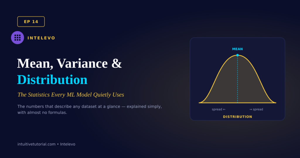
A distribution simply describes how often each value shows up across your entire dataset. Line up every value, and one shape appears again and again in nature: a peak in the middle, with both sides thinning out toward the edges. You already know this shape by its nickname — the bell curve.
heights = np.random.normal(loc=165, scale=8, size=1000)
# → most people cluster near 165cm, fewer show up at the extremes
Picture a mountain instead of a formula. The peak marks where most values sit. The slopes show how quickly the numbers thin out as you move away from that peak. That’s a distribution, and that’s really all it is.
Why Shape Matters More Than People Expect
Here’s why this final idea deserves your attention. A value sitting far out on the thin edge of a distribution is called an outlier, and outliers cause real trouble.
prices = np.array([210000, 245000, 198000, 4500000])
print(np.mean(prices))
# → one huge outlier drags the "typical" price way up
That single unusual price distorts the mean instantly. Worse, many machine learning models quietly assume your data roughly follows a bell curve. So the moment your data’s real shape breaks that assumption, your model’s performance can break right along with it. Checking the shape first protects you from that surprise.
Common Mistakes Learners Make With These Three Ideas
Before we combine everything, let’s clear up a few mix-ups that trip up beginners constantly. Avoiding these early saves you real debugging time later.
Mistake one: trusting the mean alone. A single average never tells the full story. Always pair it with variance before you draw a conclusion from it. Otherwise, you risk missing wildly different groups hiding behind one identical number.
Mistake two: confusing variance with standard deviation. Variance squares the differences from the mean, so its units get squared too. Standard deviation simply takes the square root of variance, which brings the units back to something readable. In practice, most people reach for np.std() because it’s easier to interpret directly.
Mistake three: ignoring the shape entirely. Two datasets can share the same mean and the same variance, yet still look completely different once you plot them. One might cluster symmetrically, while another piles up on one side with a long tail. Always glance at a histogram before you trust your summary numbers.
Mistake four: assuming every dataset is “normal.” Not every distribution follows a bell curve. Income data, for instance, usually skews heavily to one side, because a small number of very high earners pull the tail rightward. Assuming normality when it doesn’t apply can quietly break your model’s assumptions.
Once you internalize these four traps, you’ll read any dataset summary with far more confidence.
Putting the Three Ideas Together
Let’s connect everything, because these three ideas rarely work alone. In practice, a data scientist almost always checks center, spread, and shape together, right at the start of any project.
import numpy as np

prices = np.array([210000, 245000, 198000, 500000, 230000])

center = np.mean(prices)     # MEAN: the typical value
spread = np.std(prices)      # VARIANCE: how scattered the values are
shape  = "right-skewed"      # DISTRIBUTION: a few high values pull it right

print(center, spread, shape)
Three lines. Three ideas. One honest snapshot of an entire dataset. That’s the real power of mean, variance, and distribution working as a team.
A Quick Side-by-Side Recap
Before we move on, here’s a fast summary you can bookmark:
| Concept | What It Is | Analogy | In One Line |
|---|---|---|---|
| Mean | A single typical value | The balancing point | np.mean() |
| Variance | How scattered the values are | An elastic band, tight or loose | np.var() / np.std() |
| Distribution | The overall shape of the values | A mountain’s peak and slopes | A histogram’s shape |
Test Yourself: Does It Click Yet?
Here’s a quick gut-check question, straight from the video. Two neighborhoods share the exact same average home price. Neighborhood A has low variance. Neighborhood B has high variance. What does that tell you about Neighborhood B?
Take a moment before you scroll further.
The answer: prices in Neighborhood B swing much more widely, some far below average and some far above it. Same mean, completely different story. That’s variance doing exactly what it’s meant to do.
You’ve Already Seen This Math Everywhere
At this point, you might assume this math stays locked inside data science. It doesn’t. You encounter it constantly, often without noticing:
- Grading on a curve. Teachers lean on the class mean and spread to decide who lands above or below average.
- A/B testing. Companies compare the mean result across two groups to decide which version genuinely wins.
- Weather forecasts. A “70% chance of rain” comes directly from the distribution of past, similar days.
- Stock market swings. Volatility is simply another name for variance, tracked day after day.
So the next time a headline mentions an average, a spread, or a trend, you’ll recognize exactly what sits underneath it.
Where This Fits Into Your Machine Learning Journey
Let’s zoom out for a second. Earlier episodes in this series covered vectors, matrices, and dot products — the structural language every model speaks. This episode adds the statistical language: mean, variance, and distribution.
Together, these two toolkits already explain most of what happens inside model.fit() and model.predict(). And that combination sets up the next natural step perfectly.
Coming Up Next: Probability for ML
In Episode 15, we’ll build on this foundation with probability, conditional probability, and Bayes’ theorem. Put simply, we’ll explore how a model updates its guess the instant new evidence arrives. And just like this episode, we’ll explain it the same simple way, one idea at a time.
Frequently Asked Questions
Do I need calculus to understand mean, variance, and distribution? No. Every idea in this article uses basic arithmetic and a single NumPy function. Calculus explains where these formulas come from, but you don’t need it to use them well.
Which one should I check first on a new dataset? Start with the mean, then check variance right after. Together they give you a fast center-and-spread summary. Finally, plot a histogram so you can confirm the shape matches what those two numbers suggest.
Does variance or standard deviation matter more in practice? Standard deviation usually wins for everyday interpretation, since it shares the same units as your original data. Variance still matters mathematically, though, especially inside formulas used during model training.
Can a dataset have a normal distribution but still contain outliers? Yes, and this happens often. Even well-behaved, bell-shaped data can contain a few rare extreme values. That’s exactly why checking the shape doesn’t replace checking for outliers separately.
Final Thoughts
Mean, variance, and distribution don’t have to feel like exam-day math. Once you see them as three questions — where’s the center, how spread out is it, and what shape does it take — they turn into common sense fast.
So next time you load a dataset, run these three checks first. Your future models will thank you for it.
If this breakdown helped things click, watch the full video walkthrough above, and subscribe to Intelevo for the rest of this series. Drop your questions in the comments below — every one gets read.
This article accompanies Episode 14 of the Intelevo YouTube series, “Statistics Refresher: Mean, Variance & Distributions.” Follow along at intuitivetutorial.com for the full Machine Learning roadmap, code, and companion articles for every episode.